B.2 Selected discrete distributions of random variables

B.2.1 Binomial distribution

The binomial distribution is a useful model for binary decisions where the outcome is a choice between two alternatives (e.g., Yes/No, Left/Right, Present/Absent, Heads/Tails, …). The two outcomes are coded as \(0\) (failure) and \(1\) (success). Consequently, let the probability of occurrence of the outcome “success” be \(p\), then the probability of occurrence of “failure” is \(1-p\). Consider a coin-flip experiment with the outcomes “heads” or “tails”. If we flip a coin repeatedly, e.g., 30 times, the successive trials are independent of each other and the probability \(p\) is constant, then the resulting binomial distribution is a discrete random variable with outcomes \(\{0,1,2,...,30\}\).
The binomial distribution has two parameters “size” and “prob”, often denoted as \(n\) and \(p\), respectively. The “size” parameter refers to the number of trials and “prob” to the probability of success: \[X \sim Binomial(n,p).\]

Figure B.15 shows the probability mass function of three binomially distributed random variables with different parameter values. As stated above, \(p\) refers to the probability of success. The higher this probability, the more often we will observe the outcome coded with “1”. Therefore, the distribution tends toward the right side and vice-versa. The distribution gets more symmetric if the parameter \(p\) approximates 0.5. Figure B.16 shows the corresponding cumulative functions.

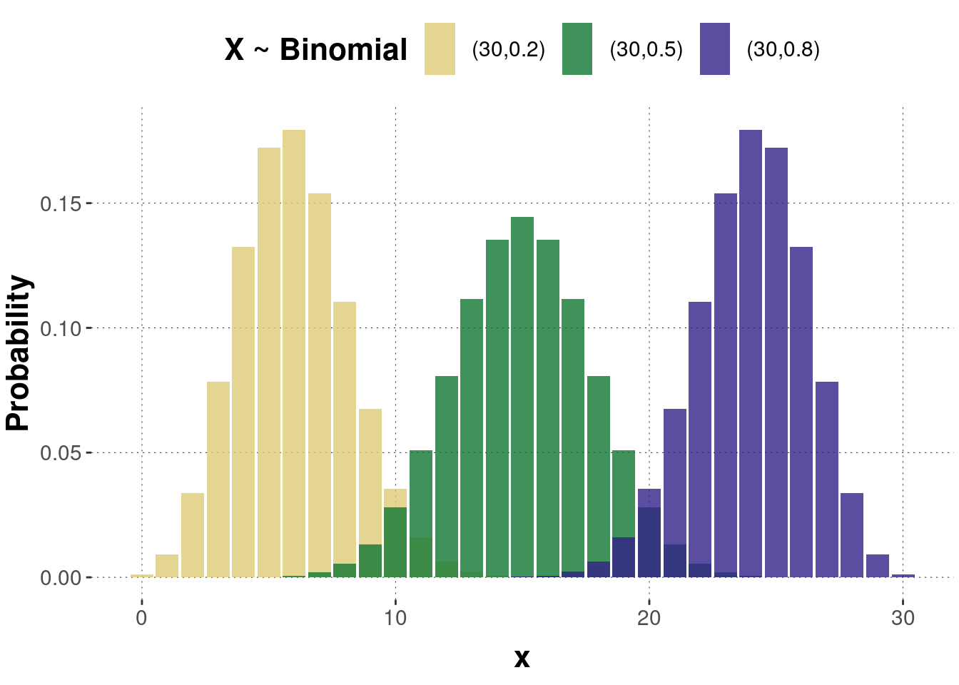
Figure B.15: Examples of a probability mass function of the binomial distribution. Numbers in the legend are pairs of parameters \((n, p)\).

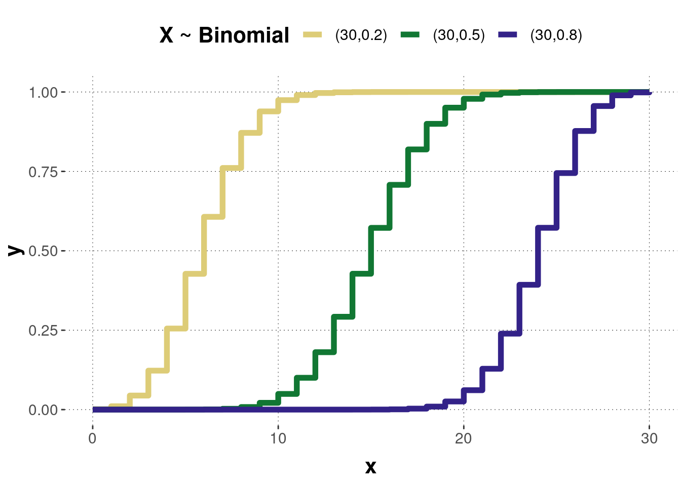
Figure B.16: The cumulative distribution functions of the binomial distributions corresponding to the previous probability mass functions.

Probability mass function

\[f(x)=\binom{n}{x}p^x(1-p)^{n-x},\] where \(\binom{n}{x}\) is the binomial coefficient.

Cumulative function

\[F(x)=\sum_{k=0}^{x}\binom{n}{k}p^k(1-p)^{n-k}\]

Expected value \(E(X)=n \cdot p\)

Variance \(Var(X)=n \cdot p \cdot (1-p)\)

B.2.1.1 Hands-on

Here’s WebPPL code to explore the effect of different parameter values on a binomial distribution:

var p = 0.5;           // probability of success
var n = 4;             // number of trials (>= 1)
var n_samples = 30000; // number of samples used for approximation
///fold:
viz(repeat(n_samples, function(x) {binomial({p: p, n: n})}));
///

B.2.2 Multinomial distribution

The multinomial distribution is a generalization of the binomial distribution to the case of \(n\) repeated trials: While the binomial distribution can have two outcomes, the multinomial distribution can have multiple outcomes. Consider an experiment where each trial can result in any of \(k\) possible outcomes with a probability \(p_i\), where \(i=1,2,...,k\), with \(\sum_{i=1}^kp_i=1\). For \(n\) repeated trials, let \(k_i\) denote the number of times \(X=x_i\) was observed, where \(i=1,2,...,m\). It follows that \(\sum_{i=1}^m k_i=n\).

Probability mass function

The probability of observing a vector of outcomes \(\mathbf{k}=[k_1,...,k_m]^T\) is

\[f(\mathbf{k}|\mathbf{p})=\binom{n}{k_1\cdot k_2 \cdot...\cdot k_m} \prod_{i=1}^m p_i^{k_i},\]

where \(\binom{n}{k_1\cdot k_2 \cdot...\cdot k_m}\) is the multinomial coefficient: \[\binom{n}{k_1\cdot k_2 \cdot...\cdot k_m}=\frac{n!}{k_1!\cdot k_2! \cdot...\cdot k_m!}.\] It is a generalization of the binomial coefficient \(\binom{n}{k}\).

Expected value: \(E(X)=n\cdot p_i\)

Variance: \(Var(X)=n\cdot p_i\cdot (1-p_i)\)

B.2.2.1 Hands-on

Here’s WebPPL code to explore the effect of different parameter values on a multinomial distribution:

var ps = [0.25, 0.25, 0.25, 0.25];  // probabilities
var n = 4;                          // number of trials (>= 1)
var n_samples = 30000;              // number of samples used for approximation
///fold:
viz.hist(repeat(n_samples, function(x) {multinomial({ps: ps, n: n})}));
///

B.2.3 Bernoulli distribution

The Bernoulli distribution is a special case of the binomial distribution with \(size = 1\). The outcome of a Bernoulli random variable is therefore either 0 or 1. Apart from that, the same information holds as for the binomial distribution. As the “size” parameter is now negligible, the Bernoulli distribution has only one parameter, the probability of success \(p\): \[X \sim Bern(p).\] Figure B.17 shows the probability mass function of three Bernoulli distributed random variables with different parameters. Figure B.18 shows the corresponding cumulative distributions.

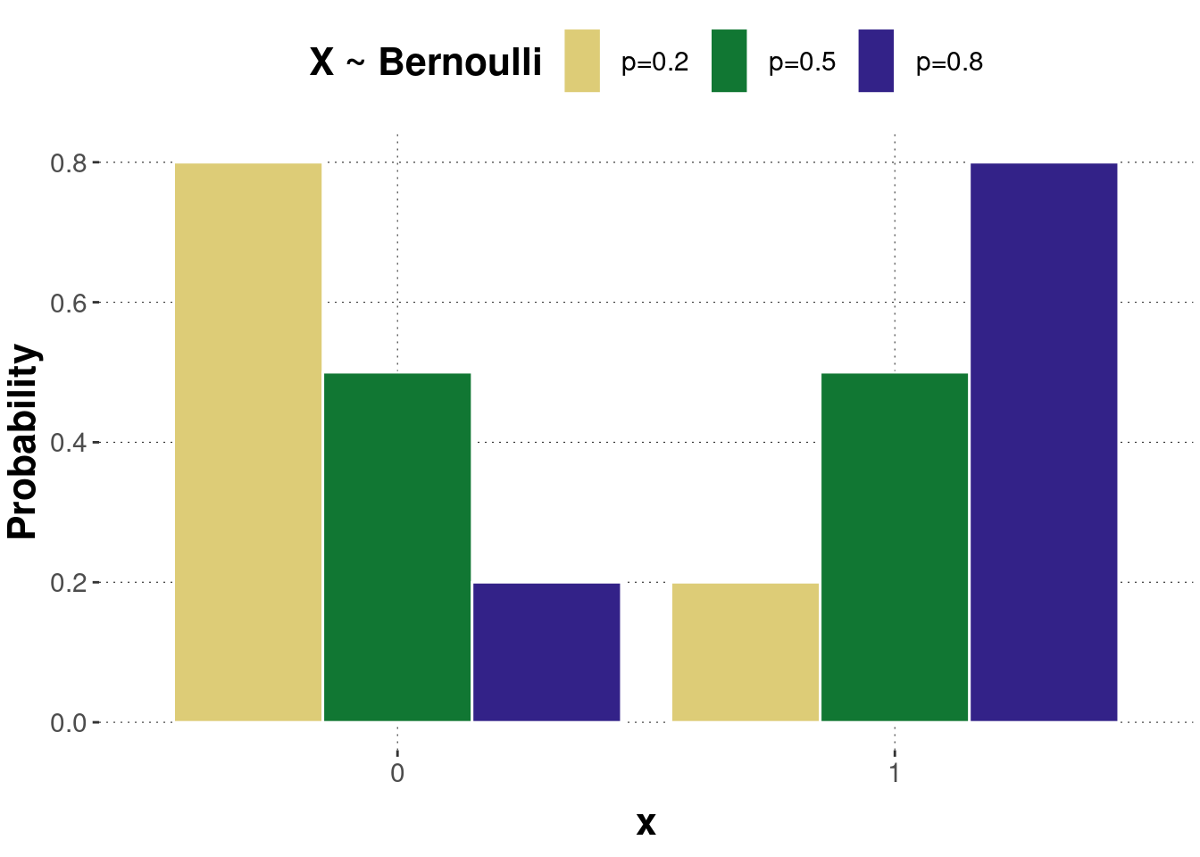
Figure B.17: Examples of a probability mass function of the Bernoulli distribution.

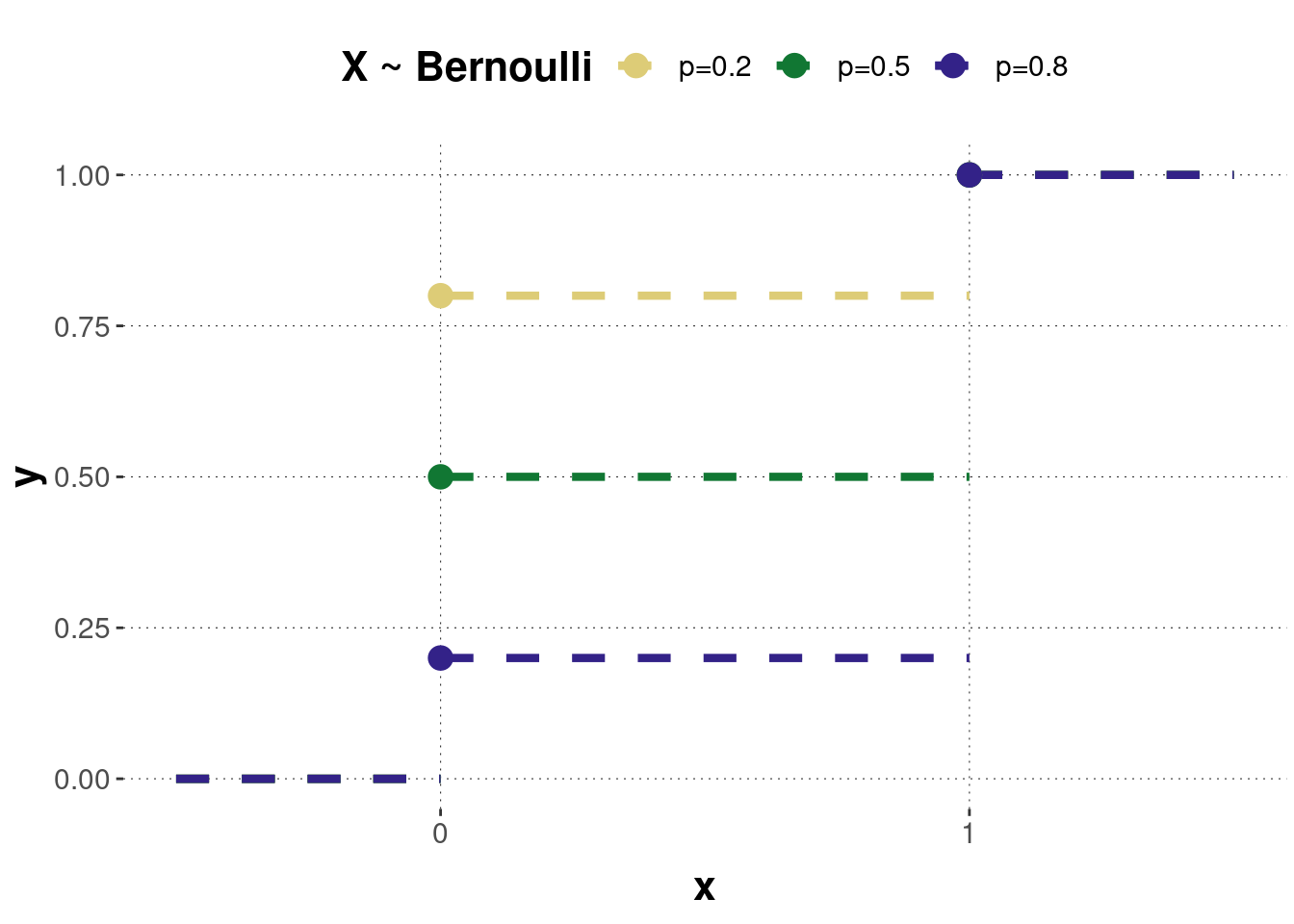
Figure B.18: The cumulative distribution functions of the Bernoulli distributions corresponding to the previous probability mass functions.

Probability mass function

\[f(x)=\begin{cases} p &\textrm{ if } x=1,\\ 1-p &\textrm{ if } x=0.\end{cases}\]

Cumulative function

\[F(x)=\begin{cases} 0 &\textrm{ if } x < 0, \\ 1-p &\textrm{ if } 0 \leq x <1,\\1 &\textrm{ if } x \geq 1.\end{cases}\]

Expected value \(E(X)=p\)

Variance \(Var(X)=p \cdot (1-p)\)

B.2.3.1 Hands-on

Here’s WebPPL code to explore the effect of different parameter values on a Bernoulli distribution:

var p = 0.5;           // probability of success
var n_samples = 30000; // number of samples used for approximation
///fold:
viz(repeat(n_samples, function(x) {bernoulli({p: p})}));
///

B.2.4 Categorical distribution

The categorical distribution is a generalization of the Bernoulli distribution for categorical random variables: While a Bernoulli distribution is a distribution over two alternatives, the categorical is a distribution over multiple alternatives. For a single trial (e.g., a single die roll), the categorical distribution is equal to the multinomial distribution.

The categorical distribution is parametrized by the probabilities assigned to each event. Let \(p_i\) be the probability assigned to outcome \(i\). The set of \(p_i\)’s are the parameters, constrained by \(\sum_{i=1}^kp_i=1\).

\[X \sim Categorical(\mathbf{p})\]

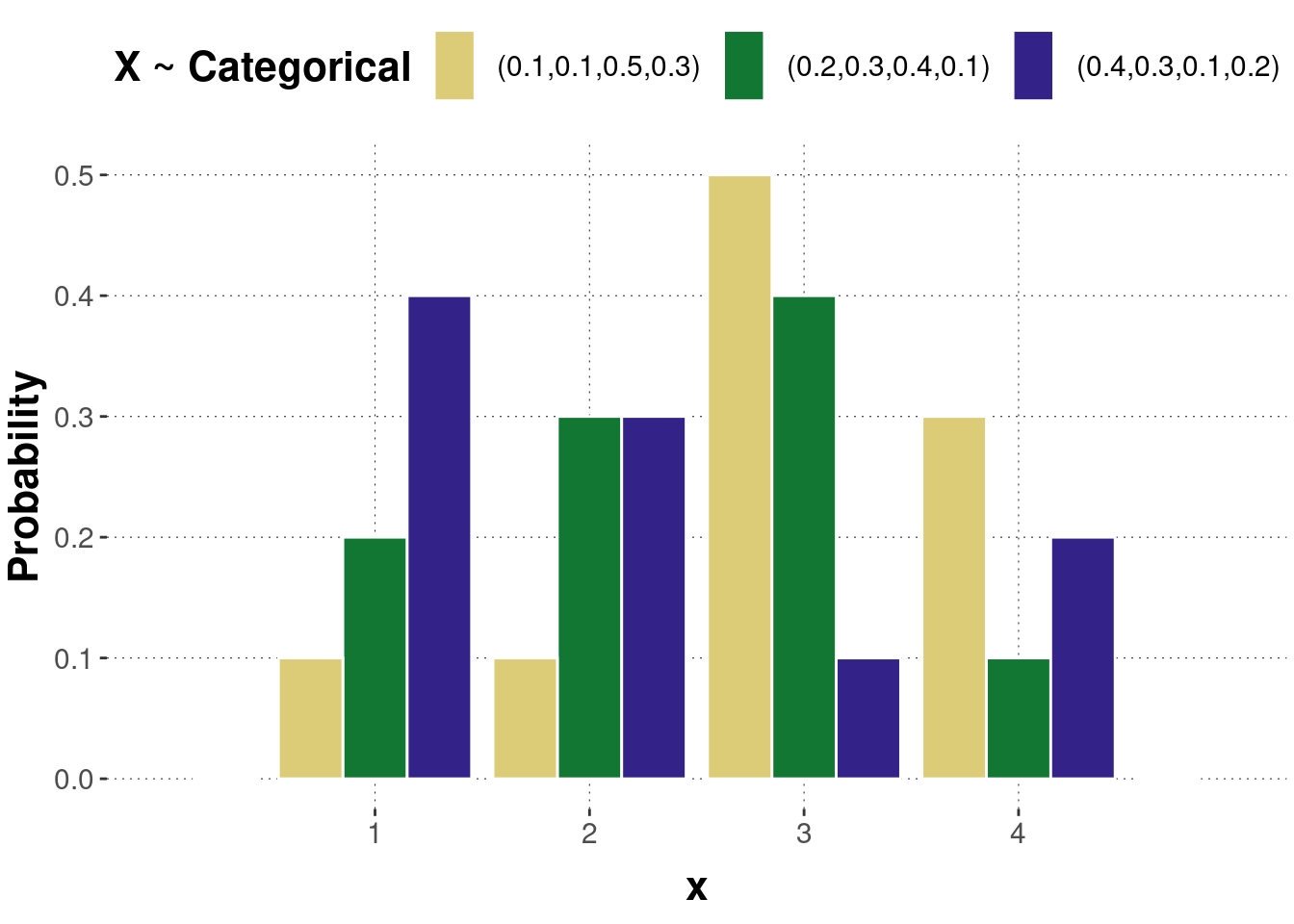
Figure B.19: Examples of a probability mass function of the categorical distribution.

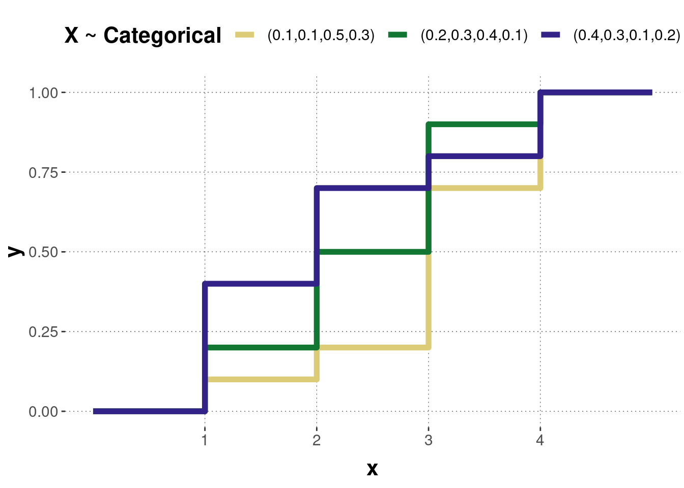
Figure B.20: The cumulative distribution functions of the categorical distributions corresponding to the previous probability mass functions.

Probability mass function

\[f(x|\mathbf{p})=\prod_{i=1}^kp_i^{\{x=i\}},\]

where \(\{x=i\}\) evaluates to 1 if \(x=i\), otherwise 0 and \(\mathbf{p}={p_1,...,p_k}\), where \(p_i\) is the probability of seeing event \(i\).

Expected Value \(E(\mathbf{x})=\mathbf{p}\)

Variance \(Var(\mathbf{x})=\mathbf{p}\cdot(1-\mathbf{p})\)

B.2.4.1 Hands-on

Here’s WebPPL code to explore the effect of different parameter values on a categorical distribution:

var ps = [0.5, 0.25, 0.25];  // probabilities
var vs = [1, 2, 3];          // categories
var n_samples = 30000;       // number of samples used for approximation
///fold:
viz(repeat(n_samples, function(x) {categorical({ps: ps, vs: vs})}));
///

B.2.5 Beta-Binomial distribution

As the name already indicates, the beta-binomial distribution is a mixture of a binomial and beta distribution. Remember, a binomial distribution is useful to model a binary choice with outcomes “0” and “1”. The binomial distribution has two parameters \(p\) and \(n\), denoting the probability of success (“1”) and the number of trials, respectively. Furthermore, we assume that the successive trials are independent and \(p\) is constant. In a beta-binomial distribution, \(p\) is not anymore assumed to be constant (or fixed) but changes from trial to trial. Thus, a further assumption about the distribution of \(p\) is made, and here the beta distribution comes into play: the probability \(p\) is assumed to be randomly drawn from a beta distribution with parameters \(a\) and \(b\). Therefore, the beta-binomial distribution has three parameters \(n\), \(a\) and \(b\): \[X \sim BetaBinom(n,a,b).\] For large values of a and b, the distribution approaches a binomial distribution. When \(a=1\) and \(b=1\), the distribution equals a discrete uniform distribution from 0 to \(n\). When \(n = 1\), the distribution equals a Bernoulli distribution.

Figure B.21 shows the probability mass function of three beta-binomial distributed random variables with different parameter values. Figure B.22 shows the corresponding cumulative distributions.

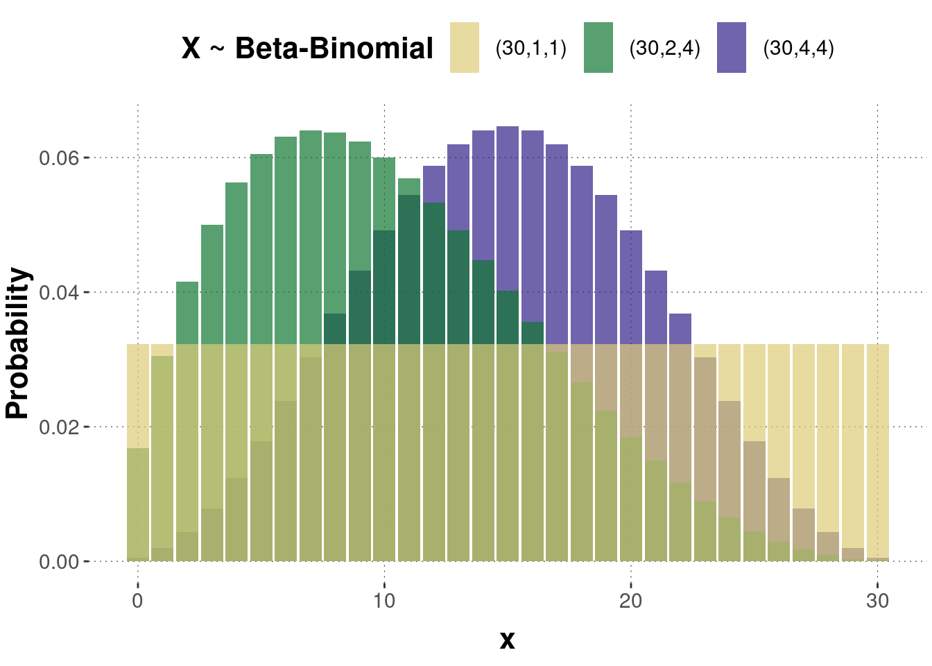
Figure B.21: Examples of a probability mass function of the beta-binomial distribution. Triples of numbers in the legend represent parameter values \((n,a,b)\).

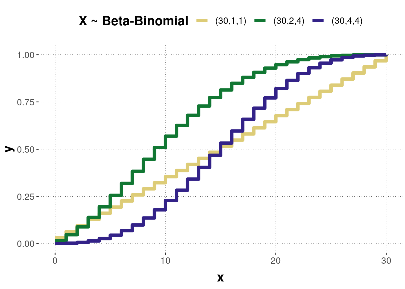
Figure B.22: The cumulative distribution functions of the beta-binomial distributions corresponding to the previous probability mass functions.

Probability mass function

\[f(x)=\binom{n}{x} \frac{B(a+x,b+n-x)}{B(a,b)},\]

where \(\binom{n}{x}\) is the binomial coefficient and \(B(x)\) is the beta function (see beta distribution).

Cumulative function

\[F(x)=\begin{cases} 0 &\textrm{ if } x<0,\\ \binom{n}{x} \frac{B(a+x,b+n-x)}{B(a,b)} {}_3F_2(n,a,b) &\textrm{ if } 0 \leq x < n,\\ 1 &\textrm{ if } x \geq n. \end{cases}\] where \({}_3F_2(n,a,b)\) is the generalized hypergeometric function.

Expected value \(E(X)=n \frac{a}{a+b}\)

Variance \(Var(X)=n \frac{ab}{(a+b)^2} \frac{a+b+n}{a+b+1}\)

B.2.5.1 Hands-on

Here’s WebPPL code to explore the effect of different parameter values on a beta-binomial distribution:

var a = 1;              // shape parameter alpha
var b = 1;              // shape parameter beta
var n = 10;             // number of trials (>= 1)
var n_samples = 30000;  // number of samples used for approximation
///fold:
viz(repeat(n_samples, function(x) {binomial({n: n, p: beta(a, b)})}));
///

B.2.6 Poisson distribution

A Poisson distributed random variable represents the number of events occurring in a given time interval. The Poisson distribution is a limiting case of the binomial distribution when the number of trials becomes very large and the probability of success is small (e.g., the number of car accidents in Osnabrueck in the next month, the number of typing errors on a page, the number of interruptions generated by a CPU during T seconds, etc.). Events described by a Poisson distribution must fulfill the following conditions: they occur in non-overlapping intervals, they do not occur simultaneously, and each event occurs at a constant rate.

The Poisson distribution has one parameter, the rate \(\lambda\), sometimes also referred to as intensity:

\[X \sim Poisson(\lambda).\]

The parameter \(\lambda\) can be thought of as the expected number of events in the time interval. Consequently, changing the rate parameter changes the probability of seeing different numbers of events in one interval. Figure B.23 shows the probability mass function of three Poisson distributed random variables with different parameter values. Notice that the higher \(\lambda\), the more symmetrical the distribution gets. In fact, the Poisson distribution can be approximated by a normal distribution for a rate parameter of \(\geq\) 10. Figure B.24 shows the corresponding cumulative distributions.

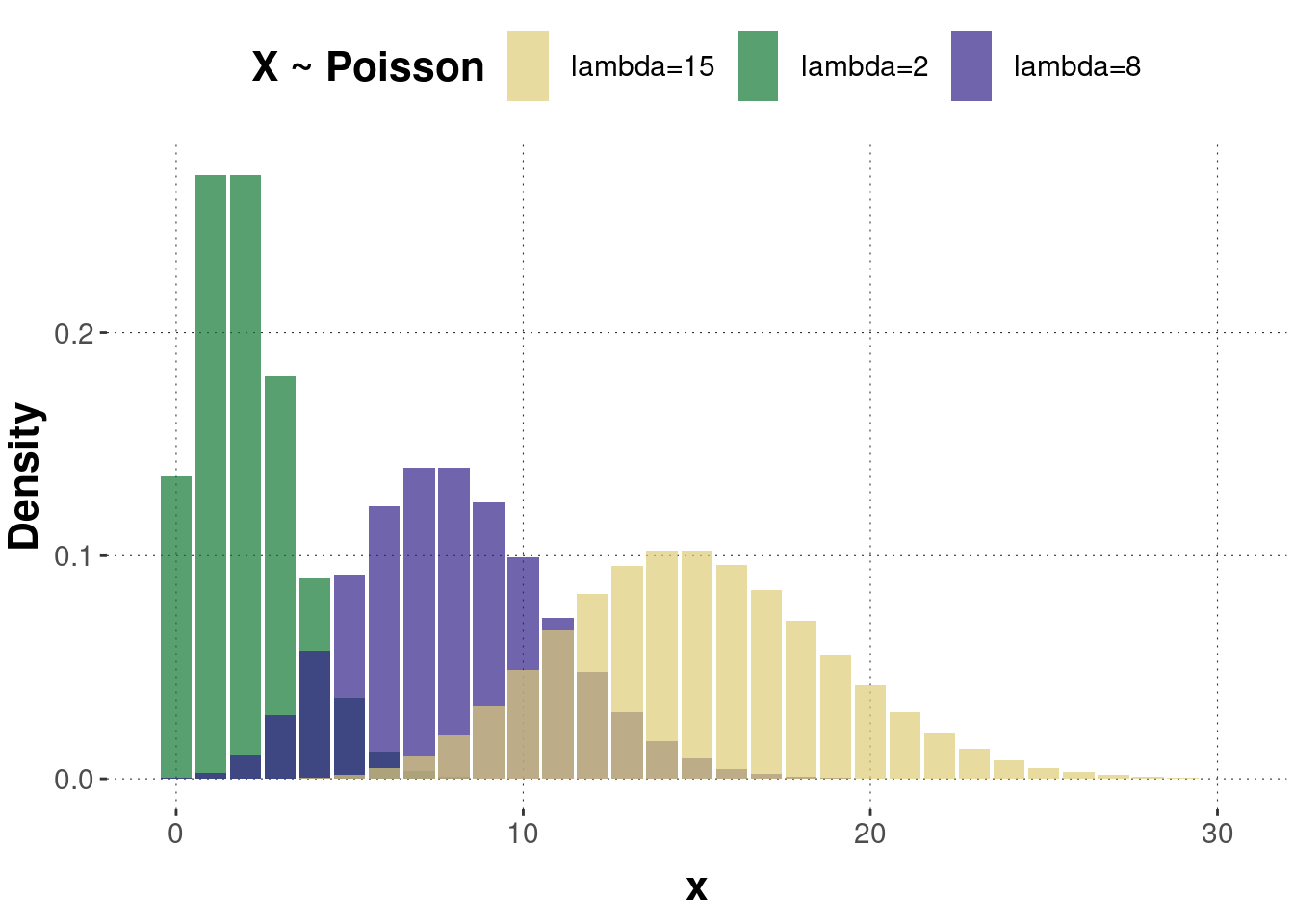
Figure B.23: Examples of a probability mass function of the Poisson distribution.

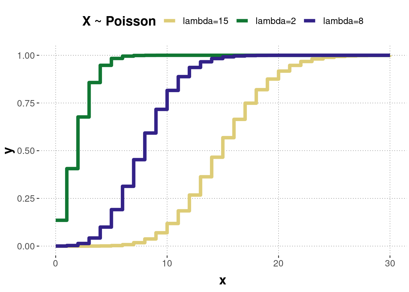
Figure B.24: The cumulative distribution functions of the Poisson distributions corresponding to the previous probability mass functions.

Probability mass function

\[f(x)=\frac{\lambda^x}{x!}e^{-\lambda}\]

Cumulative function

\[F(x)=\sum_{k=0}^{x}\frac{\lambda^k}{k!}e^{-\lambda}\]

Expected value \(E(X)= \lambda\)

Variance \(Var(X)=\lambda\)

B.2.6.1 Hands-on

Here’s WebPPL code to explore the effect of different parameter values on a Poisson distribution:

var lambda = 5;        // rate parameter
var n_samples = 30000; // number of samples used for approximation
///fold:
viz(repeat(n_samples, function(x) {poisson({mu: lambda})}));
///