At the end of the previous section, we saw that we can use the AIC-approach to calculate an approximate value of the posterior probability \(P(M_{i} \mid D)\) for model \(M_{i}\) given data \(D\). The Bayes factor approach is similar to this, but avoids taking priors over models into the equation by focusing on the extent to which data \(D\) changes our beliefs about which model is more likely.
Take two Bayesian models:
\(M_1\) has prior \(P(\theta_1 \mid M_1)\) and likelihood \(P(D \mid \theta_1, M_1)\)
\(M_2\) has prior \(P(\theta_2 \mid M_2)\) and likelihood \(P(D \mid \theta_2, M_2)\)
Using Bayes rule, we compute the posterior odds of models (given the data) as the product of the likelihood ratio and the prior odds.
The likelihood ratio is also called the Bayes factor. Formally, the Bayes factor is the factor by which a rational agent changes her prior odds in the light of observed data to arrive at the posterior odds. More intuitively, the Bayes factor quantifies the strength of evidence given by the data about the models of interest. It expresses this evidence in terms of the models’ relative prior predictive accuracy. To see the latter, let’s expand the Bayes factor as what it actually is: the ratio of marginal likelihoods.
Three insights are to be gained from this expansion. Firstly, the Bayes factor is a measure of how well each model would have predicted the data ex ante, i.e., before having seen any data. In this way, it is diametrically opposed to a concept like AIC, which relies on models’ maximum likelihood fits (therefore using the data, so being ex post).
Secondly, the marginal likelihood of a model is exactly the quantity that we identified (in the context of parameter estimation) as being very hard to compute, especially for complex models. The fact that marginal likelihoods are hard to compute was the reason that methods like MCMC sampling are useful, since they give posterior samples without requiring the calculation of marginal likelihoods.
It follows that Bayes factors can be very difficult to compute in general.
However, for many prominent models, it is possible to calculate Bayes factors analytically if the right kinds of priors are specified (Rouder et al. 2009; Rouder and Morey 2012; Gronau, Ly, and Wagenmakers 2019).
We will see an example of this in Chapter 11.
Also, as we will see in the following there are very clever approaches to computing Bayes factors in special cases and good algorithms for approximating marginal likelihoods also for complex models.
Thirdly, Bayes factor model comparison implicitly (and quite vigorously) punishes model complexity, but in a more sophisticated manner than just counting free parameters. To appreciate this intuitively, imagine a model with a large parameter set and a very diffuse, uninformative prior that spreads its probability over a wide range of parameter values. Since Bayes factors are computed based on ex ante predictions, a diffuse model is punished for its imprecision of prior predictions because we integrate over all parameters (weighted by priors) and their associated likelihood.
As for notation, we write:
\[\text{BF}_{12} = \frac{P(D \mid M_1)}{P(D \mid M_2)}\]
for the Bayes factor in favor of model \(M_1\) over model \(M_2\). This quantity can take on positive values, which are often translated into natural language as follows:
\(BF_{12}\)
interpretation
1
irrelevant data
1 - 3
hardly worth ink or breath
3 - 6
anecdotal
6 - 10
now we’re talking: substantial
10 - 30
strong
30 - 100
very strong
100 +
decisive (bye, bye \(M_2\)!)
As \(\text{BF}_{12} = \text{BF}_{21}^{-1}\), it suffices to give this translation into natural language only for values \(\ge 1\).
Bayes Factors have a nice property: We can retrieve the Bayes Factor for models \(M_{0}\) and \(M_{2}\) when we know the Bayes Factors of \(M_{0}\) and \(M_{2}\) each to another model \(M_{1}\).
Proposition 10.1 ('Transitivity' of Bayes Factors) For any three models \(M_{0}\), \(M_{1}\), and \(M_{2}\): \(\mathrm{BF}_{02} = \mathrm{BF}_{01} \ \mathrm{BF}_{12}\).
Proof. For any two models \(M_{i}\) and \(M_{j}\), the Bayes Factor \(\mathrm{BF}_{ij}\) is given as the factor by which the prior odds and the posterior odds differ:
\[\begin{align*}
% \label{eq:observation-BF-1}
\mathrm{BF}_{ij} = \frac{P(M_{i} \mid D)}{P(M_{j} \mid D)} \frac{P(M_{j})}{P(M_{i})}\,,
\end{align*}\]
which can be rewritten as:
\[\begin{align*}
% \label{eq:observation-BFs-2}
\frac{P(M_{i} \mid D)}{P(M_{i})} = \mathrm{BF}_{ij} \frac{P(M_{j} \mid D)}{P(M_{j})}\,.
\end{align*}\]
Using these observations, we find that:
\[\begin{align*}
\mathrm{BF}_{02}
& = \frac{P(M_{0} \mid D)}{P(M_{2} \mid D)} \frac{P(M_{2})}{P(M_{0})}
= \frac{P(M_{0} \mid D)}{P(M_{0})} \frac{P(M_{2})}{P(M_{2} \mid D)}
\\
& = \mathrm{BF}_{01} \frac{P(M_{1} \mid D)}{P(M_{1})} \ \frac{1}{\mathrm{BF}_{21}} \frac{P(M_{1}) }{P(M_{1} \mid D)}
= \mathrm{BF}_{01} \ \mathrm{BF}_{12}
\end{align*}\]
There are at least two general approaches to calculating or approximating Bayes factors, paired here with a (non-exhaustive) list of example methods:
We can use grid approximation to approximate a model’s marginal likelihood if the model is small enough, say, no more than 4-5 free parameters.
Grid approximation considers discrete values for each parameter evenly spaced over the whole range of plausible parameter values, thereby approximating the integral in the definition of marginal likelihoods.
Let’s calculate an example for the comparison of the exponential and the power model of forgetting.
To begin with, we need to define a prior over parameters to obtain Bayesian versions of the exponential and power model.
Here, we assume flat priors over a reasonable range of parameter values for simplicity. For the exponential model, we choose:
To approximate each model’s marginal likelihood via grid approximation, we consider equally spaced values for both parameters (a tighly knit grid), assess the prior and likelihood for each parameter pair and finally take the sum over all of the visited values:
# make sure the functions accept vector inputlhExp <-Vectorize(lhExp)lhPow <-Vectorize(lhPow)# define the step size of the gridstepsize <-0.01# calculate the marginal likelihoodmarg_lh <-expand.grid(x =seq(0.005, 1.495, by = stepsize),y =seq(0.005, 1.495, by = stepsize)) %>%mutate(lhExp =lhExp(x, y), priExp =1/length(x), # uniform priors!lhPow =lhPow(x, y), priPow =1/length(x) )# output resultstr_c("BF in favor of exponential model: ", with(marg_lh, sum(priExp * lhExp) /sum(priPow * lhPow)) %>%round(2))
## [1] "BF in favor of exponential model: 1221.39"
Based on this computation, we would be entitled to conclude that the data provide overwhelming evidence in favor of the exponential model. The result tells us that a rational agent should adjust her prior odds by a factor of more than 1000 in favor of the exponential model when updating her beliefs with the data. In other words, the data tilt our beliefs very strongly towards the exponential model, no matter what we believed initially. In this sense, the data provide strong evidence for the exponential model.
10.3.2 Naive Monte Carlo
For simple models (with maybe 4-5 free parameters), we can also use naive Monte Carlo sampling to approximate Bayes factors. In particular, we can approximate the marginal likelihood by taking samples from the prior, calculating the likelihood of the data for each sampled parameter tuple, and then averaging over all calculated likelihoods:
Here is a calculation using one million samples from the prior of each model:
nSamples <-1000000# sample from the priora <-runif(nSamples, 0, 1.5)b <-runif(nSamples, 0, 1.5)# calculate likelihood of data for each samplelhExpVec <-lhExp(a, b)lhPowVec <-lhPow(a, b)# compute marginal likelihoodsstr_c("BF in favor of exponential model: ", round(mean(lhExpVec) /mean(lhPowVec), 2))
## [1] "BF in favor of exponential model: 1218.39"
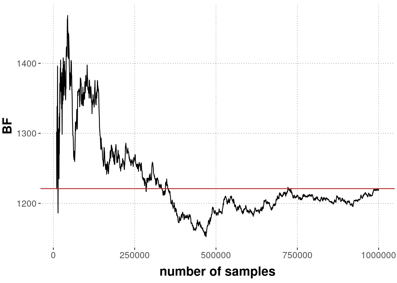
We can also check the time course of our MC-estimate by a plot like that in Figure 10.3.
The plot shows the current estimate of the Bayes factor on the \(y\)-axis after having taken the number of samples given on the \(x\)-axis.
We see that the initial calculations (after only 10,000 samples) are far off, but that the approximation finally gets reasonably close to the value calculated by grid approximation, which is shown as the red line.
Figure 10.3: Temporal development (as more samples come in) of the Monte Carlo estimate of the Bayes factor in favor of the exponential model over the power model of forgetting. The red horizontal line indicates the Bayes factor estimate obtained previously via grid approximation.
Exercise 11.3
Which statements concerning Bayes Factors (BF) are correct?
The Bayes Factor shows the absolute probability of a particular model to be a good explanation of the observed data.
If \(BF_{12} = 11\), one should conclude that there is strong evidence in favor of \(M_1\).
Grid approximation allows us to compare no more than five models simultaneously.
With the Naive Monte Carlo method, we can only approximate the BF for models with continuous parameters.
BF computation penalizes more complex models.
Statements b. and e. are correct.
10.3.3 Excursion: Bridge sampling
For more complex models (e.g., high-dimensional/hierarchical parameter spaces), naive Monte Carlo methods can be highly inefficient. If random sampling of parameter values from the priors is unlikely to deliver values for which the likelihood of the data is reasonably high, most naive MC samples will contribute very little information to the overall estimate of the marginal likelihood. For this reason, there are better sampling-based procedures which preferentially sample a posteriori credible parameter values (given the data) and use clever math to compensate for using the wrong distribution to sample from. This is the main idea behind approaches like importance sampling. A very promising approach is in particular bridge sampling, which also has its own R package (Gronau et al. 2017).
We will not go into the formal details of this method, but just showcase here an application of the bridgesampling package.
This approach requires samples from the posterior, which we can obtain using Stan (see Section 9.3.2).
Towards this end, we first assemble the data for input to the Stan program in a list:
forgetting_data <-list(N =100,k = obs,t = t)
The models are implemented in Stan. We here only show the exponential model.
data {
  int<lower=1> N ;
  int<lower=0,upper=N> k[6] ;
  int<lower=0> t[6];
}
parameters {
  real<lower=0,upper=1.5> a ;
  real<lower=0,upper=1.5> b ;
}
model {
  // likelihood
  for (i in 1:6) {
    target += binomial_lpmf(k[i] | N,  a * exp(-b * t[i])) ;
  }
}
We then use Stan to obtain samples from the posterior in the usual way. To get reliable estimates of Bayes factors via bridge sampling, we should take a much larger number of samples than we usually would for a reliable estimation of, say, the posterior means and credible intervals.
stan_fit_expon <- rstan::stan(# where is the Stan codefile ='models_stan/model_comp_exponential_forgetting.stan',# data to supply to the Stan programdata = forgetting_data,# how many iterations of MCMCiter =20000,# how many warmup stepswarmup =2000)
stan_fit_power <- rstan::stan(# where is the Stan codefile ='models_stan/model_comp_power_forgetting.stan',# data to supply to the Stan programdata = forgetting_data,# how many iterations of MCMCiter =20000,# how many warmup stepswarmup =2000)
The bridgesampling package can then be used to calculate each model’s marginal likelihood.
We then obtain an estimate of the Bayes factor in favor of the exponential model with this function:
bridgesampling::bf(expon_bridge, power_bridge)
## Estimated Bayes factor in favor of expon_bridge over power_bridge: 1220.25382
References
Gronau, Quentin F., Alexander Ly, and Eric-Jan Wagenmakers. 2019. “Informed Bayesian t-Tests.”The American Statistician.
Gronau, Quentin F., Alexandra Sarafoglou, Dora Matzke, Alexander Ly, Udo Boehm, Maarten Marsman, David S. Leslie, Jonathan J. Forster, Eric-Jan Wagenmakers, and Helen Steingroever. 2017. “A Tutorial on Bridge Sampling.”Journal of Mathematical Psychology 81: 80–97.
Rouder, Jeffrey N., and Richard D. Morey. 2012. “Default Bayes Factors for Model Selection in Regression.”Multivariate Behavioral Research 47 (6): 877–903.
Rouder, Jeffrey N., Paul l. Speckman, Dongchu Sun, Richard D. Morey, and Geoffrey Iverson. 2009. “Bayesian t Tests for Accepting and Rejecting the Null Hypothesis.”Psychonomic Bulletin & Review 16 (2): 225–37.