The general logic of Bayesian hypothesis testing via parameter estimation is this.
Let \(M\) be the assumed model for observed data \(D_{\text{obs}}\).
We use Bayesian posterior inference to calculate or approximate the posterior \(P_M(\theta \mid M)\).
We then look at an interval-based estimate, most usually a Bayesian credible interval, and compare the hypothesis in question to the region of a posteriori most probable values for the parameter(s) targeted by the hypothesis.
Concretely, for point-valued hypotheses we can use the following approach. Let \(\Theta\) be the parameter space of a model \(M\). We are interested in some component \(\Theta_i\) and our hypothesis is \(\Theta_i = \theta^*_i\) for some specific value \(\theta^*_i\). A simple (but crude and controversial) way of addressing this point-valued hypothesis based on observed data \(D\) is to look at whether \(\theta^*_i\) lies inside some credible interval for parameter \(\Theta_i\) in the posterior derived by updating with data \(D\). A customary choice here are 95% credible intervals, but also other choices, e.g., 80% credible intervals, are used.
If a categorical decision rule is needed, we can:
accept the point-valued hypothesis if \(\theta^*\) is inside of the credible interval; and
reject the point-valued hypothesis if \(\theta^*\) is outside of the credible interval.
Kruschke (2015) extends this approach to also address ROPE-d hypotheses. He argues that we should not be concerned with point-valued hypotheses, but rather with intervals constructed around the point-value of interest. Kruschke, therefore, suggests looking at a region of practical equivalence (ROPE), usually defined by some \(\epsilon\)-region around \(\theta^*_i\):
The choice of \(\epsilon\) is context-dependent and requires an understanding of the scale at which parameter values \(\Theta_i\) differ. If the parameter of interest is, for example, a difference \(\delta\) in the means of reaction times, like in the Simon task, this parameter is intuitively interpretable. We can say, for instance, that an \(\epsilon\)-region of \(\pm 15\text{ms}\) is really so short that any value in \([-15\text{ms}; 15\text{ms}]\) would be regarded as identical to \(0\) for all practical purposes because of what we know about reaction times and their potential differences. However, with parameters that are less clearly anchored to a concrete physical measurement about which we have solid distributional knowledge and/or reliable intuitions, fixing the size of the ROPE can be more difficult. For the bias of a coin flip, for instance, which we want to test at the point value \(\theta^* = 0.5\) (testing the coin for fairness), we might want to consider a ROPE like \([0.49; 0.51]\), although this choice may be less objectively defensible without previous experimental evidence from similar situations.
In Kruschke’s ROPE-based approach where \(\epsilon > 0\), the decision about a point-valued hypothesis becomes ternary. If \([l;u]\) is an interval-based estimate of parameter \(\Theta_i\) and \([\theta^*_i - \epsilon; \theta^*_i + \epsilon]\) is the ROPE around the point-value of interest, we would:
accept the point-valued hypothesis iff \([l;u]\) is contained entirely in \([\theta^*_i - \epsilon; \theta^*_i + \epsilon]\);
reject the point-valued hypothesis iff \([l;u]\) and \([\theta^*_i - \epsilon; \theta^*_i + \epsilon]\) have no overlap; and
withhold judgement otherwise.
Going beyond Kruschke’s approach to ROPE-d hypotheses, it is possible to extend this ternary decision logic also to cover directional hypotheses.
11.3.1 Example: 24/7
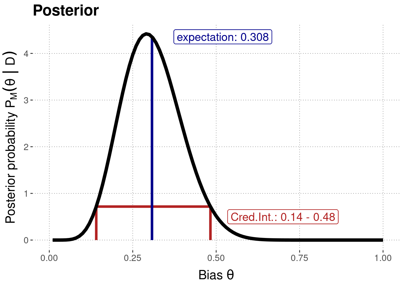
For the Binomial model and the 24/7 data, we know that the posterior is of the form \(\text{Beta}(8,18)\).
Here is a plot of the posterior (repeated from before) which also includes the 95% credible interval for the coin bias \(\theta_c\).
To address our point-valued hypothesis of \(\theta_{c} = 0.5\) that the coin is fair, we just have to check if the critical value of 0.5 is inside or outside the 95% credible interval.
In the case at hand, it is not.
We would therefore, by the binary decision logic of this approach, reject the hypothesis \(\theta_{c} = 0.5\) that the coin is fair.
(Notice that while, strictly speaking, this approach does not pay attention to how closely the credible interval includes or excludes the critical value, we should normally take into account that the boundaries of the credible intervals are uncertain estimates based on posterior samples.)
Using the ROPE-approach of Kruschke, we notice that our ROPE of \(\theta = 0.5 \pm 0.01\) is also fully outside of the 95% HDI.
Here too, we conclude that the idea of an “approximately fair coin” is sufficiently unlikely to act as if it was false.
In other words, by the ternary decision logic of this approach, we would reject the ROPE-d hypothesis \(\theta = 0.5 \pm 0.01\).
(In practice, especially when we are uncertain about how exactly to pin down \(\epsilon\), we might also sometimes want to give the range of \(\epsilon\) values for which the ROPE-d hypothesis would be accepted or rejected. So, here we could also say that for any \(\epsilon < 0.016\) we would reject the ROPE-d hypothesis.)
The directional hypothesis that the coin is biased towards tails \(\theta_c < 0.5\) contains the 95% credible interval in its entirety.
We would therefore, following the ternary decision logic, accept this hypothesis based on the model and data.
11.3.2 Example: Simon Task
We use Stan to draw samples from the posterior distribution.
We start with assembling the data:
# samplingstan_fit_ttest <- rstan::stan(# where is the Stan codefile ='models_stan/ttest_model.stan',# data to supply to the Stan programdata = simon_data_4_Stan,# how many iterations of MCMC # more samples b/c of following approximationsiter =20000,# how many warmup stepswarmup =1000)
Here is a concise summary of the relevant parameters:
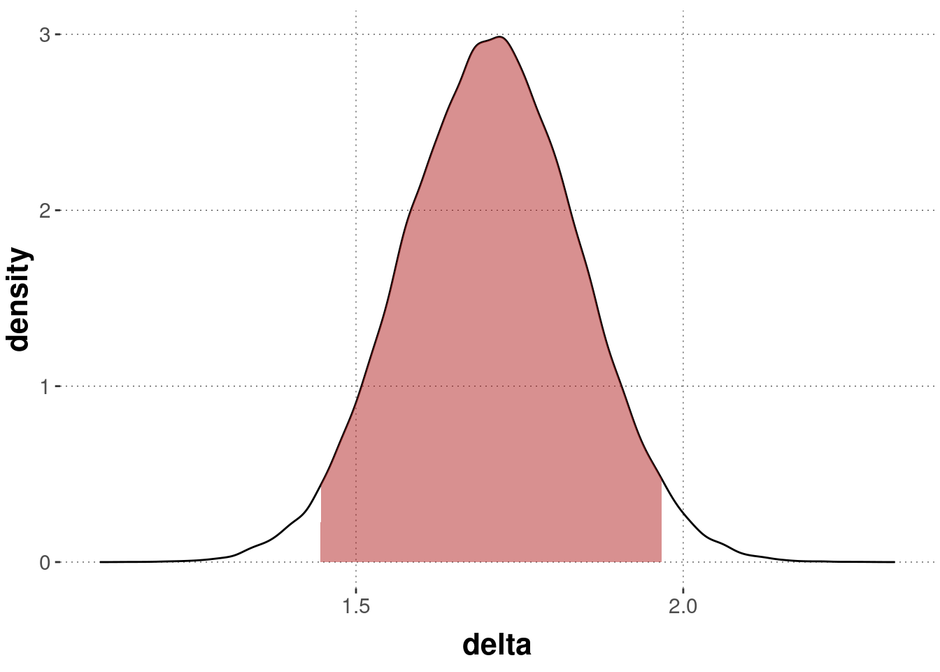
Figure 11.5 shows the posterior distribution over \(\delta\) and the 95% HDI (in red).
Figure 11.5: Posterior density of the \(\delta\) parameter in the Bayesian \(t\)-test model for Simon task data with the 95% HDI (in red).
For the point-valued estimate of \(\delta = 0\), which is clearly outside of the 95% credible interval, the binary decision criterion would have us reject the hypothesis that the difference between group means is precisely zero.
For a ROPE-d hypothesis \(\delta = 0 \pm 0.1\), we reach the same conclusion by the ternary decision rule of Kruschke, since the entire ROPE is outside of the credible interval.
The directional hypothesis that \(\delta > 0\) is accepted by the ternary decision approach.
Exercise 11.2
In this exercise, we will recap the decision rules of the two approaches introduced in this chapter. Using the binary approach for point-valued hypotheses, there are two possible outcomes, namely rejecting \(H_0\) and failing to reject \(H_0\). Following Kruschke’s ROPE approach, we can also withhold judgment. Use pen and paper to draw examples of the situations a-e given below. For each case, draw any distribution representing the posterior (e.g., a bell-shaped curve), the approximate 95% HDI and an arbitrary point value of interest \(\theta^*\). For tasks c-e, also draw an arbitrary ROPE around the point value.
Concretely, we’d like you to sketch…
…one instance where we would not reject a point-valued hypothesis \(H_0: \theta = \theta^*\).
…one instance where we would reject a point-valued hypothesis \(H_0: \theta = \theta^*\).
…two instances where we would not reject a ROPE-d hypothesis \(H_0: \theta = \theta^* \pm \epsilon\).
…two instances where we would reject a ROPE-d hypothesis \(H_0: \theta = \theta^* \pm \epsilon\).
…two instances where we would withhold judgement regarding a ROPE-d hypothesis \(H_0: \theta = \theta^* \pm \epsilon\).
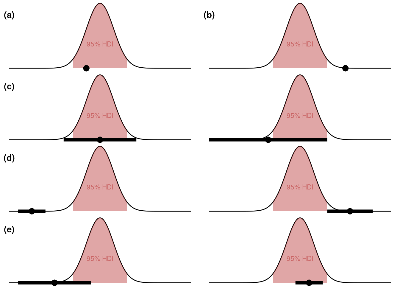
One solution to this exercise might look as follows.
The red shaded area under the curves shows the 95% credible interval. The black dots represent (arbitrary) point values of interest, and the horizontal bars in panels (c)-(e) depict the ROPE around a given point value.
References
Kruschke, John. 2015. Doing Bayesian data analysis: A tutorial with R, JAGS, and Stan. Academic Press.