D.7 Murder data
D.7.1 Nature, origin and rationale of the data
![]()
The murder data set contains information about the relative number of murders in American cities. It also contains further socio-economic information, such as a city’s unemployment rate, and the percentage of inhabitants with a low income. We use this data set just for illustration. No further real-world conclusions should be drawn from this, as the data should be treated as entirely fictitious.
murder_data <- aida::data_murderWe take a look at the data:
murder_data %>% head()## # A tibble: 6 × 4
## murder_rate low_income unemployment population
## <dbl> <dbl> <dbl> <dbl>
## 1 11.2 16.5 6.2 587000
## 2 13.4 20.5 6.4 643000
## 3 40.7 26.3 9.3 635000
## 4 5.3 16.5 5.3 692000
## 5 24.8 19.2 7.3 1248000
## 6 12.7 16.5 5.9 643000Each row in this data set shows data from a city. The information in the columns is:
murder_rate: annual murder rate per million inhabitantslow_income: percentage of inhabitants with a low income (however that is defined)unemployment: percentage of unemployed inhabitantspopulation: number of inhabitants of a city
There is information for a total of 20 cities in this data set.
Here’s a nice way of plotting each variable against each other:
GGally::ggpairs(murder_data, title = "Murder rate data")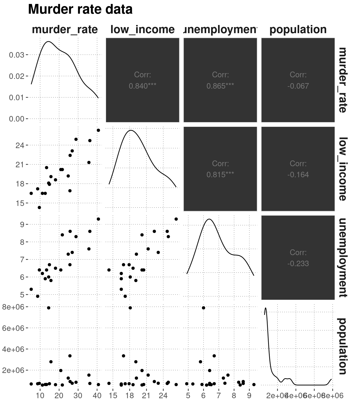
The diagonal of this graph shows the density curve of the data in each column. Scatter plots below the diagonal show pairs of values from two columns plotted against each other. The information above the diagonal gives the correlation score of each pair of variables.
The “research question” of interest for this data set is which factors help predict a city’s murder_rate.
In other words, we want to know, for example, whether knowing a random city’s value for the variable unemployment, will allow us to make better predictions about that city’s value for the variable murder_rate.
Chapter 12 uses this data set to specifically ask whether we can use information from variables like unemployment to predict murder_rate based on the assumption of a linear relationship.
It is important to stress here that asking for an epistemic / stochastic relationship of the form “Does \(x\) help to make better predictions about \(y\)?” does not relate to or presuppose a causal relationship between \(x\) and \(y\). The variables \(x\) and \(y\) could be mutual effects of a common cause, and yet still knowing about \(x\) could carry information about \(y\) even if manipulating \(x\) by divine intervention would not change \(y\), and vice versa.