D.5 Avocado prices
D.5.1 Nature, origin and rationale of the data
![]()
This data set has been plucked from Kaggle. More information on the origin and composition of this data set can be found on Kaggle’s website covering the avocado data. The data set includes information about the prices of (Hass) avocados and the amount sold (of different kinds) at different points in time. The data is originally from the Hass Avocado Board, where the data is described as follows:
The [data] represents weekly 2018 retail scan data for National retail volume (units) and price. Retail scan data comes directly from retailers’ cash registers based on actual retail sales of Hass avocados. Starting in 2013, the table below reflects an expanded, multi-outlet retail data set. Multi-outlet reporting includes an aggregation of the following channels: grocery, mass, club, drug, dollar and military. The Average Price (of avocados) in the table reflects a per unit (per avocado) cost, even when multiple units (avocados) are sold in bags. The Product Lookup codes (PLU’s) in the table are only for Hass avocados. Other varieties of avocados (e.g. greenskins) are not included in this table.
Columns of interest are:
Date: date of the observationAveragePrice: average price of a single avocadoTotal Volume: total number of avocados soldtype: whether the price/amount is for conventional or organic4046: total number of small avocados sold (PLU 4046)4225: total number of medium avocados sold (PLU 4225)4770: total number of large avocados sold (PLU 4770)
D.5.2 Loading and preprocessing the data
We load the data into a variable named avocado_data but also immediately rename some of the columns to have more convenient handles:
avocado_data <- aida::data_avocado_raw %>%
  # remove currently irrelevant columns
  select(-X1, -contains("Bags"), -year, -region) %>%
  # rename variables of interest for convenience
  rename(
    total_volume_sold = `Total Volume`,
    average_price = `AveragePrice`,
    small  = '4046',
    medium = '4225',
    large  = '4770',
  )
We can then take a glimpse:
glimpse(avocado_data)## Rows: 18,249
## Columns: 7
## $ Date <date> 2015-12-27, 2015-12-20, 2015-12-13, 2015-12-06, 201…
## $ average_price <dbl> 1.33, 1.35, 0.93, 1.08, 1.28, 1.26, 0.99, 0.98, 1.02…
## $ total_volume_sold <dbl> 64236.62, 54876.98, 118220.22, 78992.15, 51039.60, 5…
## $ small <dbl> 1036.74, 674.28, 794.70, 1132.00, 941.48, 1184.27, 1…
## $ medium <dbl> 54454.85, 44638.81, 109149.67, 71976.41, 43838.39, 4…
## $ large <dbl> 48.16, 58.33, 130.50, 72.58, 75.78, 43.61, 93.26, 80…
## $ type <chr> "conventional", "conventional", "conventional", "con…The preprocessed version of the data is stored in aida::data_avocado for later reuse.
D.5.3 Summary statistics
We are interested in the following summary statistics for the variables total_amount_sold and average_price for the whole data and for each type of avocado separately:
- mean
- median
- variance
- the bootstrapped 95% confidence interval of the mean
To get these results we define a convenience function that calculates exactly these measures:
summary_stats_convenience_fct <- function(numeric_data_vector) {
  bootstrap_results <- bootstrapped_CI(numeric_data_vector)
  tibble(
    CI_lower = bootstrap_results$lower,
    mean = bootstrap_results$mean,
    CI_upper = bootstrap_results$upper,
    median = median(numeric_data_vector),
    var = var(numeric_data_vector)
  )
}
We then apply this function once for the whole data set and once for each type of avocado (conventional or organic). We do this using a nested tibble in order to record the joint output of the convenience function (so that we only need to calculate the bootstrapped 95% confidence interval twice).
# summary stats for the whole data taken together
avocado_sum_stats_total <- avocado_data %>%
  select(type, average_price, total_volume_sold) %>%
  pivot_longer(
    cols = c(total_volume_sold, average_price),
    names_to  = 'variable',
    values_to = 'value'
  ) %>%
  group_by(variable) %>%
  nest() %>%
  summarise(
    summary_stats = map(data, function(d) summary_stats_convenience_fct(d$value))
  ) %>%
  unnest(summary_stats) %>%
  mutate(type = "both_together") %>%
  # reorder columns: moving `type` to second position
  select(1, type, everything())

# summary stats for each type of avocado
avocado_sum_stats_by_type <- avocado_data %>%
  select(type, average_price, total_volume_sold) %>%
  pivot_longer(
    cols = c(total_volume_sold, average_price),
    names_to  = 'variable',
    values_to = 'value'
  ) %>%
  group_by(type, variable) %>%
  nest() %>%
  summarise(
    summary_stats = map(data, function(d) summary_stats_convenience_fct(d$value))
  ) %>%
  unnest(summary_stats)

# joining the summary stats in a single tibble
avocado_sum_stats <-
  full_join(avocado_sum_stats_total, avocado_sum_stats_by_type)

# inspect the results
avocado_sum_stats
## # A tibble: 6 × 7
## variable type CI_lower mean CI_upper median var
## <chr> <chr> <dbl> <dbl> <dbl> <dbl> <dbl>
## 1 average_price both_together 1.40 1.41 1.41e0 1.37e0 1.62e- 1
## 2 total_volume_sold both_together 802101. 850644. 8.99e5 1.07e5 1.19e+13
## 3 average_price conventional 1.15 1.16 1.16e0 1.13e0 6.92e- 2
## 4 total_volume_sold conventional 1556392. 1653213. 1.75e6 4.08e5 2.25e+13
## 5 average_price organic 1.65 1.65 1.66e0 1.63e0 1.32e- 1
## 6 total_volume_sold organic 44920. 47811. 5.09e4 1.08e4 2.03e+10D.5.4 Plots
Here are plots of the distributions of average_price for different types of avocados:
avocado_data %>%
  ggplot(aes(x = average_price, fill = type)) +
  geom_histogram(binwidth = 0.01) +
  facet_wrap(type ~ ., ncol = 1) +
  coord_flip() +
  geom_point(
    data = avocado_sum_stats_by_type %>% filter(variable == "average_price"),
    aes(y = 0, x = mean)
  ) +
  ylab('') +
  xlab('Average price') +
  theme(legend.position = "none")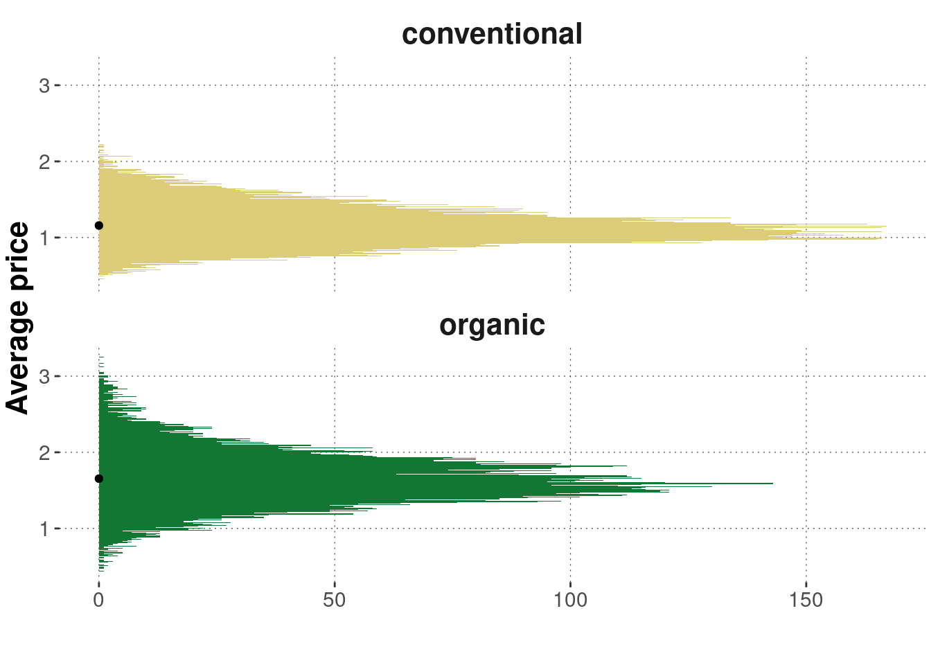
Here is a scatter plot of the logarithm of total_volume_sold against average_price:
avocado_data %>%
  ggplot(aes(x = log(total_volume_sold), y = average_price)) +
  geom_point(color = "darkgray", alpha = 0.3) +
  geom_smooth(color = "black", method = "lm") +
  xlab('Logarithm of total volume sold') +
  ylab('Average price') +
  ggtitle("Avocado prices plotted against the (log) amount sold")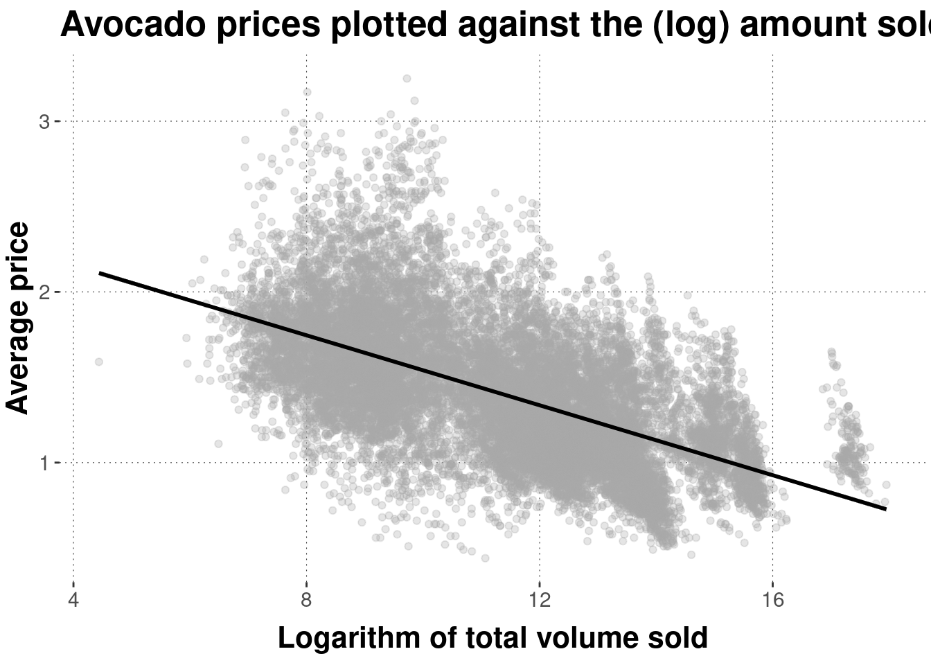
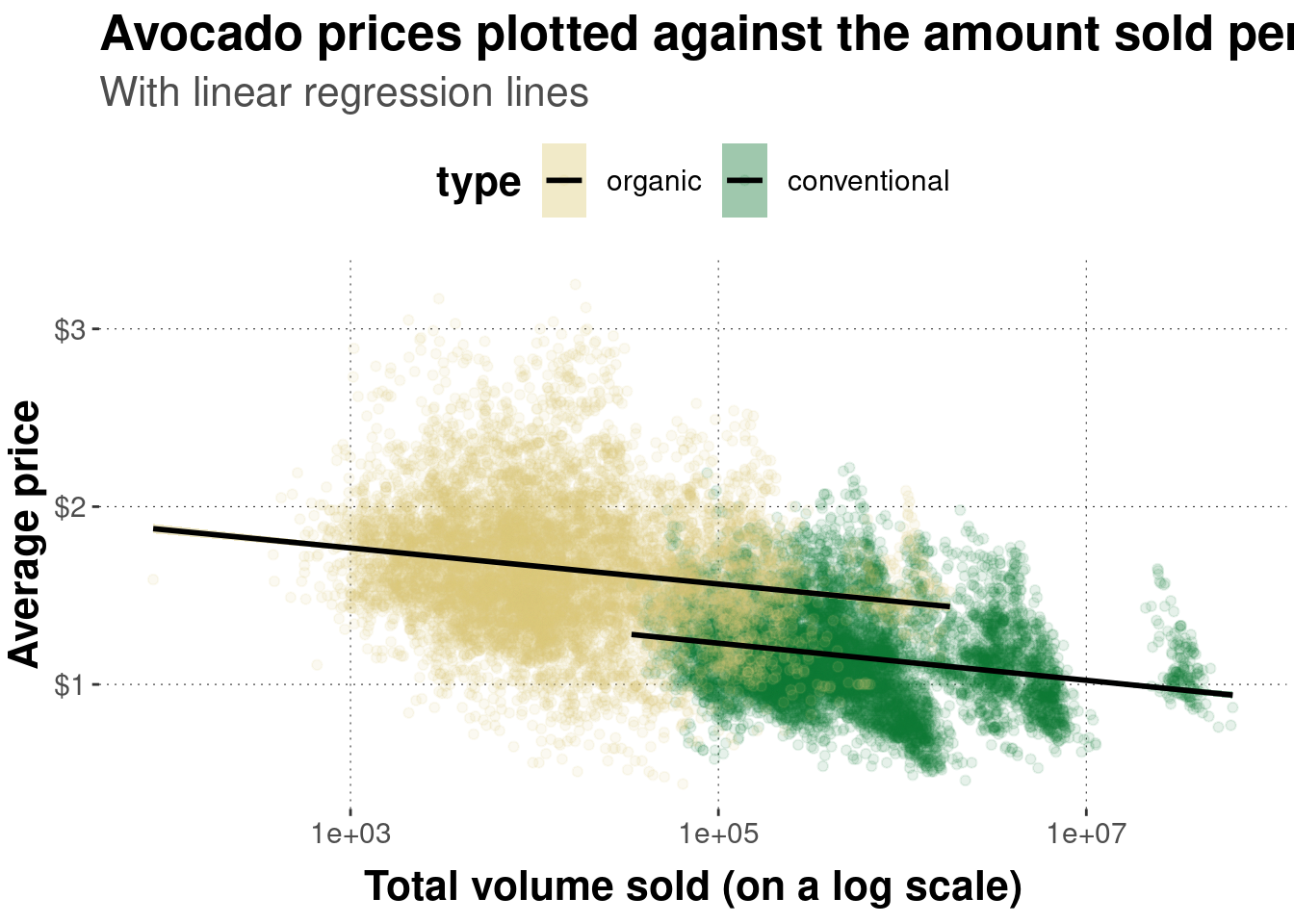
And another scatter plot, using a log-scaled \(x\)-axis and distinguishing different types of avocados:
# pipe data set into function `ggplot`
avocado_data %>%
  # reverse factor level so that horizontal legend entries align with
  # the majority of observations of each group in the plot
  mutate(
    type = fct_rev(type)
  ) %>%
  # initialize the plot
  ggplot(
    # defined mapping
    mapping = aes(
      # which variable goes on the x-axis
      x = total_volume_sold,
      # which variable goes on the y-axis
      y = average_price,
      # which groups of variables to distinguish
      group = type,
      # color and fill to change by grouping variable
      fill = type,
      color = type
    )
  ) +
  # declare that we want a scatter plot
  geom_point(
    # set low opacity for each point
    alpha = 0.1
  ) +
  # add a linear model fit (for each group)
  geom_smooth(
    color = "black",
    method = "lm"
  ) +
  # change the default (normal) of x-axis to log-scale
  scale_x_log10() +
  # add dollar signs to y-axis labels
  scale_y_continuous(labels = scales::dollar) +
  # change axis labels and plot title & subtitle
  labs(
    x = 'Total volume sold (on a log scale)',
    y = 'Average price',
    title = "Avocado prices plotted against the amount sold per type",
    subtitle = "With linear regression lines"
  )