15.1 Generalizing the linear regression model

The general architecture of a (Bayesian) generalized regression model is shown in Figure 15.1. Based on a predictor matrix \(X\) and concrete values for the regression coefficients \(\beta\), the heart of linear regression modeling is the linear predictor term:

\[ \xi = X \beta \]

The linear predictor is transformed in some way or other by what is called a link function \(LF\) to yield the predicted central tendency:

\[ \eta = LF(\xi, \theta_{LF}) \]

The link function (also sometimes specified as an inverse link function) may additionally have free model parameters \(\theta_{LF}\). The predicted central tendency \(\eta\) then serves an argument in a likelihood function \(LH\), which needs to be appropriate for the data to be explained and which, too, may have additional free model parameters \(\theta_{LH}\):

\[ y \sim LH(\eta, \theta_{LH}) \]

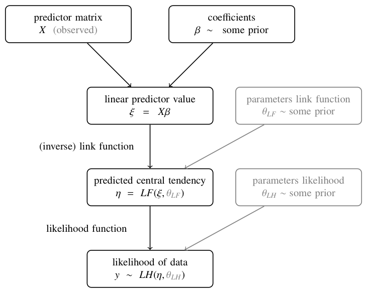
Figure 15.1: Basic architecture of generalized linear regression models.

The standard linear regression, which was covered in the previous chapters, is subsumed under this GLM scheme. To see this, consider the following representation of a (Bayesian) linear regression model:

\[ \begin{align*} \beta, \sigma & \sim \text{some prior} \\ \xi & = X \beta && \text{[linear predictor]} \\ \eta & = \xi && \text{[predictor of central tendency]} \\ y & \sim \text{Normal}(\eta, \sigma) && \text{[likelihood]} \end{align*} \] So, the standard linear regression model is the special case of the GLM scheme of Figure 15.1 in which (i) the (inverse) link function is the identity map, so that the linear predictor is the predicted central tendency \(\xi = \eta\) and (ii) the likelihood function is the normal distribution (with additional parameter \(\theta_{LF} = \sigma\)).

The need to have other likelihood functions arises when the data \(y\) to be predicted is not plausibly generated by a normal distribution. Take for instance the binary outcome of a coin flip, where a Bernoulli distribution is the natural choice for the probability of a single outcome / data observation. The Bernoulli distribution has a single parameter \(\theta_c\) (the bias of the coin), and can be written as follows, where it is assumed that \(y\) takes values 0 or 1, as usual:

\[ y \sim \text{Bernoulli}(\theta_c) = {\theta_c}^y (1- \theta_c)^{1-y} \] So, if we want a Bernoulli likelihood function (which makes perfect sense of binary outcomes) our prediction of central tendency \(\eta\) should be a latent coin bias \(\theta_c\), rather than the mean of a normal distribution. Since the coin bias is bounded \(\theta_c \in [0;1]\), but our linear predictor \(\xi \in \mathbb{R}\) is not, a link function is needed which maps (in a suitable way) a real-valued linear predictor \(\xi\) onto a bounded predictor of central tendency \(\eta = \theta_c\). Whence the need for a link function: we just need to make sure that the linear predictor (a nice, well-behaved construct) maps onto appropriate values that the likelihood function (whose nature is dictated by the (assumed) nature of the data) requires. In the case of binary data, a good choice of a link function is the logistic function. The next section looks at the resulting logistic regression model in more detail.

Other combinations of (inverse) link functions and likelihood functions give rise to other kinds of commonly used instances of generalized linear models. Below is a concise list of some of the common instances:

type of \(y\)	(inverse) link function	likelihood function
metric	\(\eta = \xi\)	\(y \sim \text{Normal}(\mu = \eta, \sigma)\)
binary	\(\eta = \text{logistic}(\xi) = (1 + \exp(-\xi))^{-1}\)	\(y \sim \text{Bernoulli}(\eta)\)
nominal	\(\eta_k = \text{soft-max}(\xi_k, \lambda) \propto \exp(\lambda \xi_k)\)	\(y \sim \text{Multinomial}({\eta})\)
ordinal	\(\eta_k = \text{threshold-Phi}(\xi_k, \sigma, {\delta})\)	\(y \sim \text{Multinomial}({\eta})\)
count	\(\eta = \exp(\xi)\)	\(y \sim \text{Poisson}(\eta)\)