16.4 [Excursion] The Neyman-Pearson approach

Neyman and Pearson criticized Fisher’s approach for not being able to deliver results that could lead to accepting the null hypothesis. Moreover, the Neynam-Pearson approach is motivated by establishing a tight regime of long-term error control: we want to keep a cap on the long-run amount of errors that we make in statistical decision making. To do so, the N-P approach requires that researchers specify not only a null hypothesis $H_0$, but also a point-valued alternative hypothesis $H_a$, which are pitted against each other (similar to what we would expect from model comparison). The point-value for $H_a$ usually comes from previous research or is chosen in a strategic manner.

If we have a pair of explicit, point-valued hypotheses, null and alternative, we can do more than just to reject or not reject the null hypothesis, so the N-P approach proposes. We can reject the null hypothesis, in which case we accept the alternative hypothesis, or we can accept the null hypothesis, in which case we reject the alternative hypothesis. Being entirely frequentist, the N-P approach makes this binary decision between competing hypotheses based on $p$-values derived from the null hypothesis, as before. As we will see, this binary accept/reject logic is only tight if we make sure that a particular kind of error, the $\beta$-error, is low enough; which we do, essentially, by making sure that we have enough data.

If we have two hypotheses $H_0$ and $H_a$, and accept/reject them in a binary fashion, there are two types of error relevant to these considerations:

the $\alpha$ or, Type-I error, is the error of falsely rejecting the null hypothesis, when in fact it is true.
the $\beta$ error, or Type-II error, is the error of falsely accepting the null hypothesis, when in fact the alternative hypothesis is true.

Figure 16.8 visualizes these two error concepts. The curves show the sampling distributions of a relevant test statistic under the assumption that $H_0$ is true (green) or that $H_a$ is true (yellow). If we fix a significance level $\alpha$ for a $p$-value based test -as before-, the proportion of error we make in the case that $H_0$ is true, is given by $\alpha$ itself. This is shown for a one-sided test in Figure 16.8, where $t^*$ is the critical value of the test statistic above which we get a significant result at $\alpha$ level. But now assume that, by the new N-P decision rule, whenever our test result is not significant, i.e., we get a result for the test statistic below $t^*$, we would accept the null hypothesis and reject the alternative hypothesis $H_a$. Then, the amount of errors we make, under the assumption that $H_a$ is actually true is given by $\beta$.

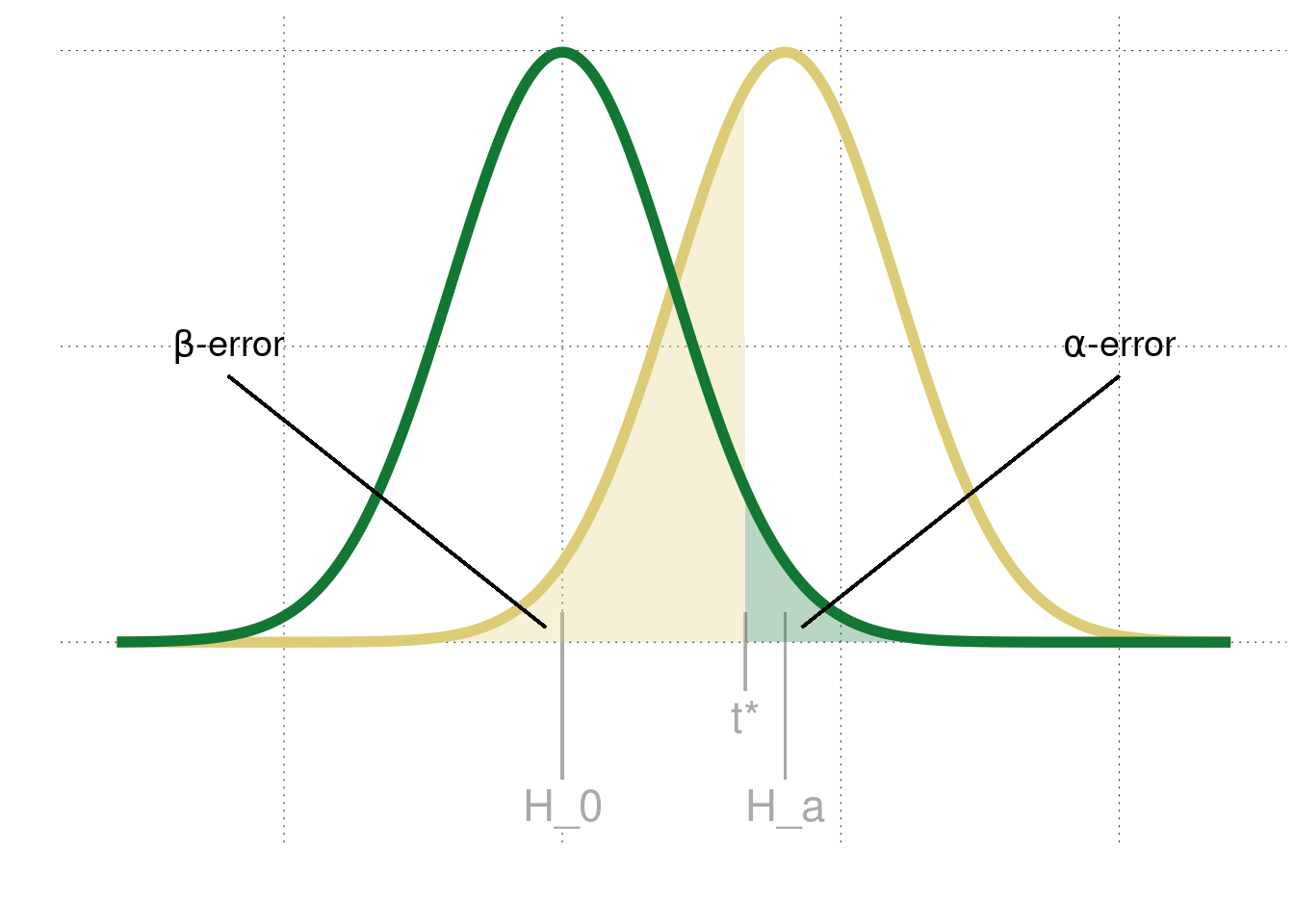
$Schematic representation of $\alpha$- and $\beta$-errors. The green curve is the sampling distribution of some test statistic under the assumption that the null hypothesis is true. The yellow curve is the sampling distribution for the alternative hypothesis. The decision criterion for an N-P test is indicated as $t^*$. The shaded regions show the probabilities of falsely rejecting a true null hypothesis (in green) and that of false accepting a false alternative hypothesis.$

Figure 16.8: Schematic representation of $\alpha$- and $\beta$-errors. The green curve is the sampling distribution of some test statistic under the assumption that the null hypothesis is true. The yellow curve is the sampling distribution for the alternative hypothesis. The decision criterion for an N-P test is indicated as $t^*$. The shaded regions show the probabilities of falsely rejecting a true null hypothesis (in green) and that of false accepting a false alternative hypothesis.

For this N-P logic of rejecting and accepting the null hypothesis to work, we would therefore need to make sure that $\beta$ is low enough. We don’t want to make that kind of mistake too often. Otherwise, we should simply withhold judgement in case of a non-significant test result.

So, how do we make sure that the $\beta$ error is small? We need to make sure that we have enough data. By the Central Limit Theorem, we know that the sampling distribution of our test statistics will have lower variance the more samples we take. Intuitively speaking, the more samples we have the steeper and tighter the curves in Figure 16.8. The $\alpha$ error will remain fixed, but the $\beta$ error decreases as the sample size increases. Consequently, if a frequentist wants to be able to both reject and accept a null hypothesis using N-P testing logic, the frequentist will:

fix $H_0$ and $H_a$ (based on previous research if possible)
determine an acceptable level of $\alpha$
determine a desired level of statistical power defined as $1-\beta$
do a power analysis, i.e., compute (using math or simulations) how many samples are necessary to meet the $1-\beta$ power bar

For simple statistical tests, like $t$-tests and ANOVA, power calculations are mathematically tractable. For more complex cases, analysts have to resort to simulations, which can be quite complex.⁸³

Power analyses are also possible for Bayesian models, but not necessary for being able to quantify evidence in favor of a null hypothesis.↩︎