D.4 Bio-Logic Jazz-Metal (and where to consume it)
D.4.1 Nature, origin and rationale of the data
![]()
This is a very short and non-serious experiment that asks for just three binary decisions from each participant, namely their spontaneous preference for one of two presented options (biology vs. logic, jazz vs. metal, and mountains vs. beach). The data from this experiment will be analyzed and plotted. This is supposed to be a useful and hopefully entertaining self-generated data set with which to practice making contingency tables and to apply binomial tests and fun stuff like that.
D.4.1.1 The experiment
D.4.1.1.1 Participants
We obtained data from 102 participants, all of whom were students of a course based on this web-book held in the winter term of 2019/2020 at the University of Osnabrück.
D.4.1.1.2 Material
There were three critical trials (and nothing else). All trials had the same trailing question:
If you have to choose between the following two options, which one do you prefer?
Each critical trial then presented two options as buttons, one of which had to be clicked.
- Biology vs. Logic
- Jazz vs. Metal
- Mountains vs. Beach
D.4.1.2 Theoretical motivation & hypotheses
This is a bogus experiment, and no sane person would advance a serious hypothesis about this. Except for the main author of this book, who conjectures that appreciators of Metal music like logic more than Jazz-enthusiasts would (because Metal is cleaner and more mechanic, while Jazz is fuzzy and organic, obviously).95
D.4.2 Loading and preprocessing the data
First, load the data:
data_BLJM_raw <- aida::data_BLJM_rawTake a peak:
glimpse(data_BLJM_raw)## Rows: 306
## Columns: 19
## $ submission_id <dbl> 379, 379, 379, 378, 378, 378, 377, 377, 377, 376, 376, 3…
## $ QUD <lgl> NA, NA, NA, NA, NA, NA, NA, NA, NA, NA, NA, NA, NA, NA, …
## $ RT <dbl> 9230, 9330, 5248, 5570, 2896, 36236, 5906, 4767, 10427, …
## $ age <dbl> 30, 30, 30, 29, 29, 29, 20, 20, 20, 21, 21, 21, 23, 23, …
## $ comments <chr> NA, NA, NA, NA, NA, NA, NA, NA, NA, NA, NA, NA, NA, NA, …
## $ education <chr> "Graduated High School", "Graduated High School", "Gradu…
## $ endTime <dbl> 1.573751e+12, 1.573751e+12, 1.573751e+12, 1.573738e+12, …
## $ experiment_id <dbl> 8, 8, 8, 8, 8, 8, 8, 8, 8, 8, 8, 8, 8, 8, 8, 8, 8, 8, 8,…
## $ gender <chr> "male", "male", "male", "male", "male", "male", "female"…
## $ languages <chr> "German", "German", "German", "German", "German", "Germa…
## $ option1 <chr> "Mountains", "Biology", "Metal", "Metal", "Biology", "Mo…
## $ option2 <chr> "Beach", "Logic", "Jazz", "Jazz", "Logic", "Beach", "Bea…
## $ question <chr> "If you have to choose between the following two options…
## $ response <chr> "Beach", "Logic", "Metal", "Metal", "Logic", "Beach", "M…
## $ startDate <chr> "Thu Nov 14 2019 18:01:24 GMT+0100 (CET)", "Thu Nov 14 2…
## $ startTime <dbl> 1.573751e+12, 1.573751e+12, 1.573751e+12, 1.573738e+12, …
## $ timeSpent <dbl> 2.3601500, 2.3601500, 2.3601500, 2.1552667, 2.1552667, 2…
## $ trial_name <chr> "forced_choice", "forced_choice", "forced_choice", "forc…
## $ trial_number <dbl> 1, 2, 3, 1, 2, 3, 1, 2, 3, 1, 2, 3, 1, 2, 3, 1, 2, 3, 1,…The most important variables in this data set are:
submission_id: unique identifier for each participantoption1andoption2: what the choice options whereresponse: which of the two options was chosen
Notice that there is no convenient column indicating which of the three critical conditions we are dealing with, so we extract that information from the data given in columns option1 and option2, while also discarding everything we will not need:96
data_BLJM_processed <-
  data_BLJM_raw %>%
  mutate(
    condition = str_c(str_sub(option2, 1, 1), str_sub(option1, 1, 1))
  ) %>%
  select(submission_id, condition, response)
data_BLJM_processed
## # A tibble: 306 × 3
## submission_id condition response
## <dbl> <chr> <chr>
## 1 379 BM Beach
## 2 379 LB Logic
## 3 379 JM Metal
## 4 378 JM Metal
## 5 378 LB Logic
## 6 378 BM Beach
## 7 377 BM Mountains
## 8 377 LB Biology
## 9 377 JM Jazz
## 10 376 BM Beach
## # … with 296 more rowsD.4.3 Exploration: counts & plots
We are interested in relevant counts of the original data, namely the number of times certain choices were made. First, let’s look at the overal choice rates in each condition:
data_BLJM_processed %>%
  # we use function`count` from the `dplyr` package
  dplyr::count(condition, response)
## # A tibble: 6 × 3
## condition response n
## <chr> <chr> <int>
## 1 BM Beach 44
## 2 BM Mountains 58
## 3 JM Jazz 64
## 4 JM Metal 38
## 5 LB Biology 58
## 6 LB Logic 44Overall it seems that mountains are preferred over beaches, Jazz is preferred over Metal and Biology is preferred over Logic.
The overall counts, however, do not tell us anything about any potentially interesting relationship between preferences. So, let’s have a closer look at the lecturer’s conjecture that a preference for logic tends to go with a stronger preference for metal than a preference for biology does. To check this, we need to look at different counts, namely the number of people who selected which music-subject pair. We collect these counts in a variable called BLJM_associated_counts:
BLJM_associated_counts <- data_BLJM_processed %>%
  select(submission_id, condition, response) %>%
  pivot_wider(names_from = condition, values_from = response) %>%
  select(-BM) %>%
  dplyr::count(JM, LB)
BLJM_associated_counts
## # A tibble: 4 × 3
## JM LB n
## <chr> <chr> <int>
## 1 Jazz Biology 38
## 2 Jazz Logic 26
## 3 Metal Biology 20
## 4 Metal Logic 18Notice that this representation is tidy, but not ideal for visual inspection. A more commonly seen format can be obtained by pivoting to a wider representation:
# visually attractive table representation
BLJM_associated_counts %>%
  pivot_wider(names_from = LB, values_from = n)
## # A tibble: 2 × 3
## JM Biology Logic
## <chr> <int> <int>
## 1 Jazz 38 26
## 2 Metal 20 18The tidy representation is ideal for plotting, though. Notice, however, that the code below plots proportions of choices, not raw counts:
BLJM_associated_counts %>%
  ggplot(aes(x = LB, y = n/sum(n), color = JM, shape = JM, group = JM)) +
  geom_point(size = 3) +
  geom_line() +
  labs(
    title = "Proportion of choices of each music+subject pair",
    x = "",
    y = ""
  )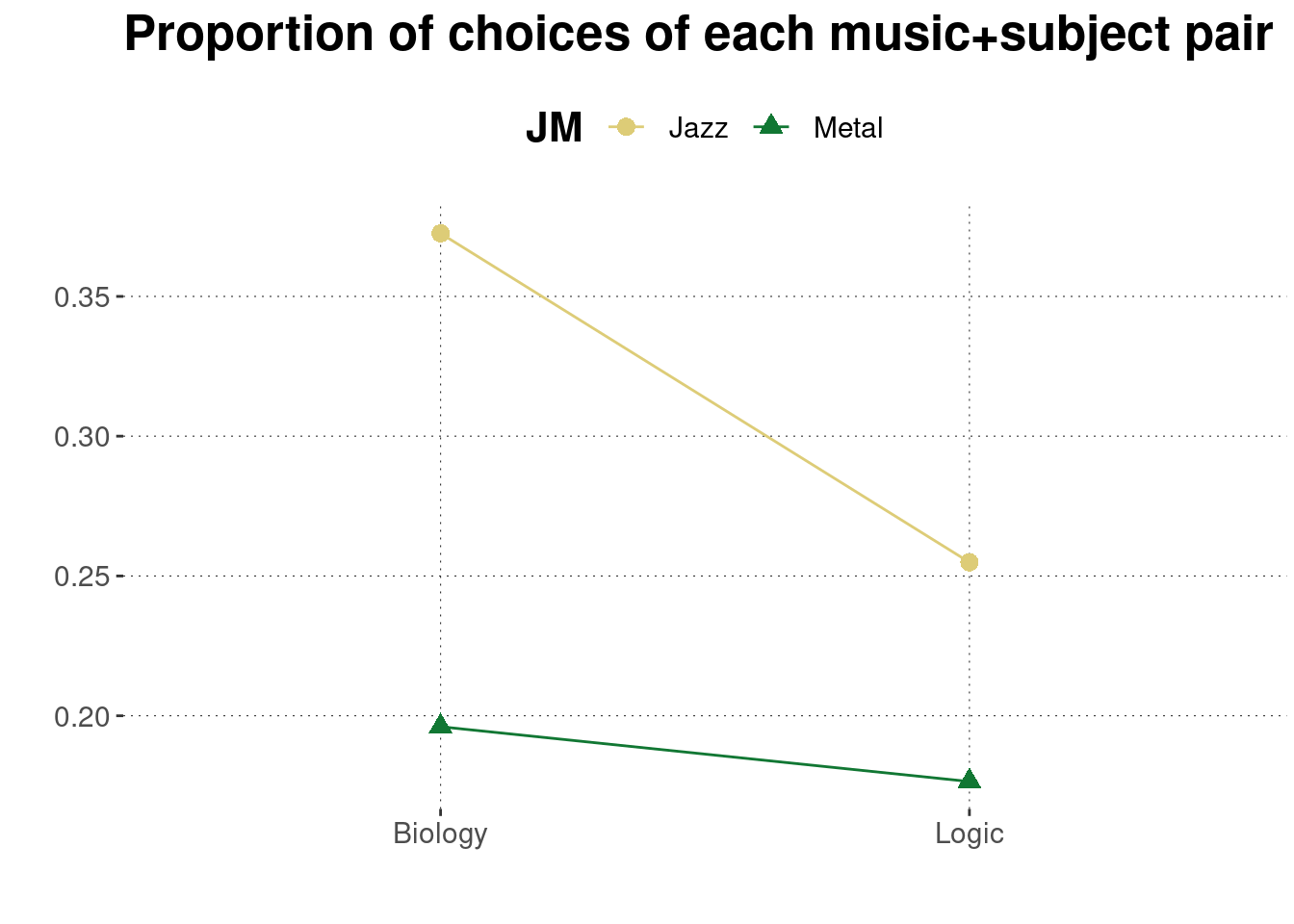
The lecturer’s conjecture might be correct. This does look like there could be an interaction. While Jazz is preferred more generally, the preference for Jazz over Metal seems more pronounced for those participants who preferred Biology than for those who preferred Logic.