6.1 Motivating example: Anscombe’s quartet
To see how summary statistics can be highly misleading, and how a simple plot can reveal a lot more, consider a famous dataset available in R (Anscombe 1973):
anscombe %>% as_tibble## # A tibble: 11 × 8
## x1 x2 x3 x4 y1 y2 y3 y4
## <dbl> <dbl> <dbl> <dbl> <dbl> <dbl> <dbl> <dbl>
## 1 10 10 10 8 8.04 9.14 7.46 6.58
## 2 8 8 8 8 6.95 8.14 6.77 5.76
## 3 13 13 13 8 7.58 8.74 12.7 7.71
## 4 9 9 9 8 8.81 8.77 7.11 8.84
## 5 11 11 11 8 8.33 9.26 7.81 8.47
## 6 14 14 14 8 9.96 8.1 8.84 7.04
## 7 6 6 6 8 7.24 6.13 6.08 5.25
## 8 4 4 4 19 4.26 3.1 5.39 12.5
## 9 12 12 12 8 10.8 9.13 8.15 5.56
## 10 7 7 7 8 4.82 7.26 6.42 7.91
## 11 5 5 5 8 5.68 4.74 5.73 6.89There are four pairs of \(x\) and \(y\) coordinates. Unfortunately, these are stored in long format with two pieces of information buried inside of the column name: for instance, the name x3 contains the information that this column contains the \(x\) coordinates for the 3rd pair. This is rather untidy. But, using tools from the dplyr package, we can tidy up quickly:
tidy_anscombe <- anscombe %>% as_tibble %>%
  pivot_longer(
    ## we want to pivot every column
    everything(),
    ## use reg-exps to capture 1st and 2nd character
    names_pattern = "(.)(.)",
    ## assign names to new cols, using 1st part of
    ##  what reg-exp captures as new column names
    names_to = c(".value", "grp")
  ) %>%
  mutate(grp = paste0("Group ", grp))
tidy_anscombe
## # A tibble: 44 × 3
## grp x y
## <chr> <dbl> <dbl>
## 1 Group 1 10 8.04
## 2 Group 2 10 9.14
## 3 Group 3 10 7.46
## 4 Group 4 8 6.58
## 5 Group 1 8 6.95
## 6 Group 2 8 8.14
## 7 Group 3 8 6.77
## 8 Group 4 8 5.76
## 9 Group 1 13 7.58
## 10 Group 2 13 8.74
## # … with 34 more rowsHere are some summary statistics for each of the four pairs:
tidy_anscombe %>%
  group_by(grp) %>%
  summarise(
    mean_x    = mean(x),
    mean_y    = mean(y),
    min_x     = min(x),
    min_y     = min(y),
    max_x     = max(x),
    max_y     = max(y),
    crrltn    = cor(x, y)
  )
## # A tibble: 4 × 8
## grp mean_x mean_y min_x min_y max_x max_y crrltn
## <chr> <dbl> <dbl> <dbl> <dbl> <dbl> <dbl> <dbl>
## 1 Group 1 9 7.50 4 4.26 14 10.8 0.816
## 2 Group 2 9 7.50 4 3.1 14 9.26 0.816
## 3 Group 3 9 7.5 4 5.39 14 12.7 0.816
## 4 Group 4 9 7.50 8 5.25 19 12.5 0.817These numeric indicators suggest that each pair of \(x\) and \(y\) values is very similar. Only the ranges seem to differ. A brilliant example of how misleading numeric statistics can be, as compared to a plot of the data:25
tidy_anscombe %>%
  ggplot(aes(x, y)) +
    geom_smooth(method = lm, se = F, color = "darkorange") +
    geom_point(color = project_colors[3], size = 2) +
    scale_y_continuous(breaks = scales::pretty_breaks()) +
    scale_x_continuous(breaks = scales::pretty_breaks()) +
    labs(
      title = "Anscombe's Quartet", x = NULL, y = NULL,
      subtitle = bquote(y == 0.5 * x + 3 ~ (r %~~% .82) ~ "for all groups")
    ) +
    facet_wrap(~grp, ncol = 2, scales = "free_x") +
    theme(strip.background = element_rect(fill = "#f2f2f2", colour = "white"))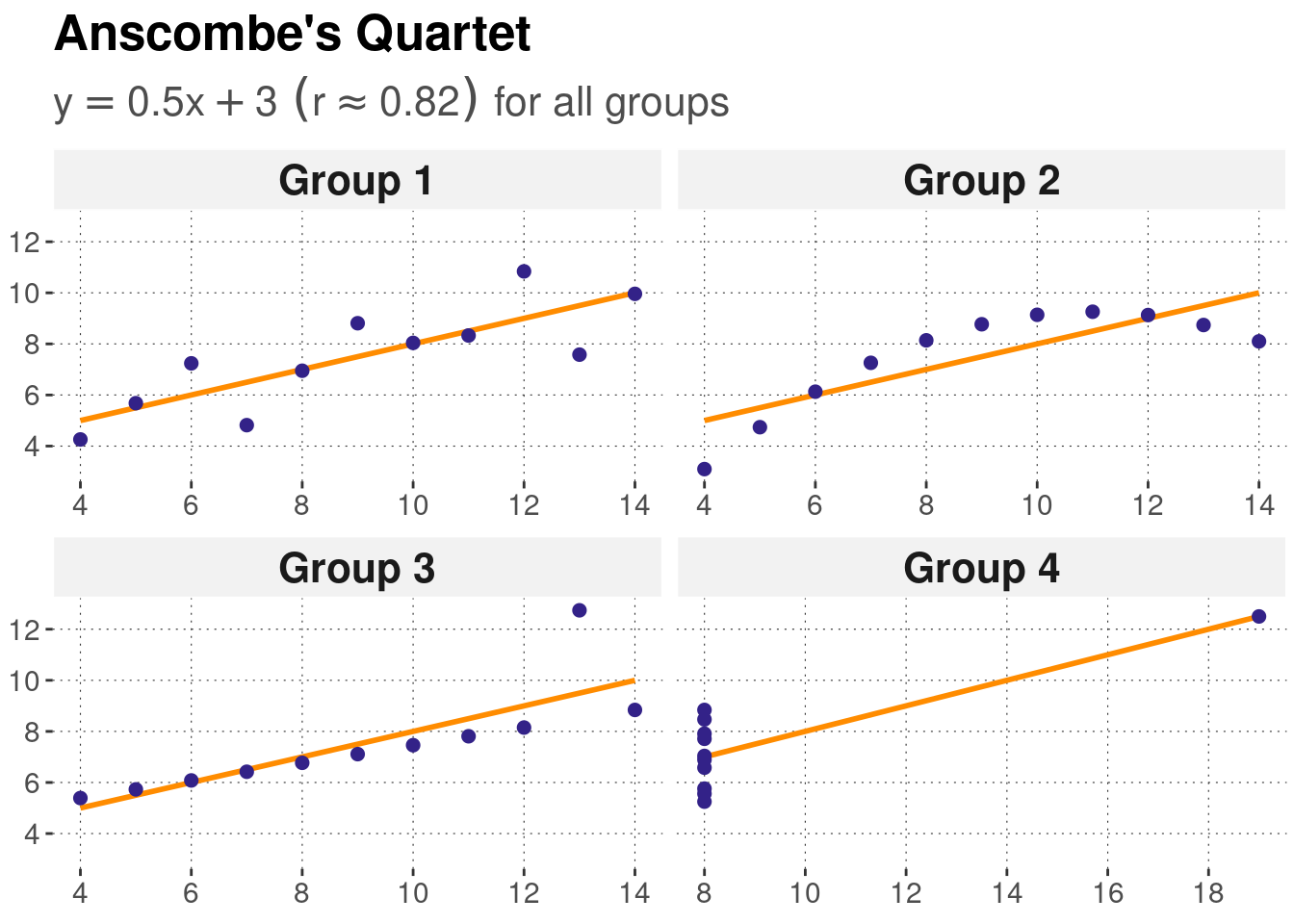
Figure 6.1: Anscombe’s Quartet: four different data sets, all of which receive the same correlation score.
References
It is not important to understand this code when you first read this chapter. But at the end of the chapter, you should be able to understand (passively) what is going on here.↩︎