17.11 Explicit beliefs vs. implicit intentions
The main objection against Bayesianism which motivated and still drives the frequentist program is that Bayesian priors are subjective, and therefore to be regarded as less scientific than hard objectively justifiable ingredients, such as likelihood functions. A modern Bayesian riposte bites the bullet, chews it well, and spits it back. While priors are subjective, they are at least explicit. They are completely out in the open and, if the data is available, predictions for any other set of prior assumptions can simply be tested. A debate about which “subjective priors” to choose is “objectively” possible. In contrast, the frequentist notion of a \(p\)-value (and with it the confidence interval) relies on something even more mystic, namely the researcher’s intentions during the data collection, something that is not even in principle openly scrutinizable after the fact. To see how central frequentist notions rely on implicit intentions and counterfactual assumptions about data we could have seen but didn’t, let’s consider an example (see also Wagenmakers (2007) and Kruschke (2015) for discussion).
The example is based on the 24/7 data again. This time, we are going to look at two cases.
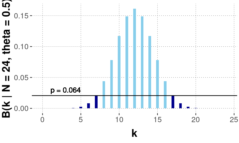
- Stop at \(N=24\): The researchers decided in advance to collect \(N=24\) data points. They found \(k=7\) heads in this experiment.
- Stop at \(k=7\): The researchers decided to flip their coin until they observed \(k=7\) heads. It took them \(N=24\) tosses in their experiment.
The research question is, as usual, whether \(\theta_c = 0.5\).
A common intuition is to say: why would the manner of data collection matter? Data is data. We base our inference on data. We don’t base our inference on how the data was obtained. Right? - Wrong if you are a frequentist.
The manner of data collection dictates what other possible observations of the experiment are. These in turn matter for computing \(p\)-values. For the “Stop at \(N=24\)” case, the likelihood function is what we used before, the Binomial distribution:
\[ \text{Binomial}(k ; n = 24, \theta = 0.5) = {{N}\choose{k}} \theta^{k} \, (1-\theta)^{n-k} \]
We therefore obtain the \(p\)-value-based result that the null hypothesis cannot be rejected (at \(\alpha = 0.05\)).
But when we look at the “Stop at \(k=7\)” case, we need a different likelihood function. In principle, we might have had to flip the coin for more than \(N=24\) times until receiving \(k=7\) heads. The likelihood function needed for this case is the negative Binomial distribution:
\[ \text{neg-Binomial}(n ; k = 7, \theta = 0.5) = \frac{k}{n} \choose{n}{k} \theta^{k} \, (1-\theta)^{n - k}\]
The resulting sampling distribution and the \(p\)-value we obtain for it are shown in the plot below.
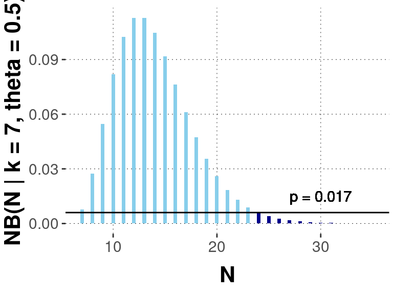
So, with the exact same data but different assumptions about how this data was generated, we get a different \(p\)-value; indeed, a difference that spans the significance boundary of \(\alpha = 0.05\). The researcher’s intentions about how to collect data influence the statistical analysis. Dependence on researcher intentions is worse than dependence on subjective priors, because it is impossible to verify ex post what the precise data-generating protocol was.
Wait! Doesn’t Bayesian inference have this problem? No, it doesn’t. The difference in likelihood functions used above is a different normalizing constant. The normalizing constant cancels out in parameter estimation, and also in model-comparison (if we assume that both models compared use the same likelihood function).92 The case of model comparison is obvious. To see that normalizing constants cancel out for parameter estimation, consider this:
\[ \begin{align*} P(\theta \mid D) & = \frac{P(\theta) \ P(D \mid \theta)}{\int_{\theta'} P(\theta') \ P(D \mid \theta')} \\ & = \frac{ \frac{1}{X} \ P(\theta) \ P(D \mid \theta)}{ \ \frac{1}{X}\ \int_{\theta'} P(\theta') \ P(D \mid \theta')} \\ & = \frac{P(\theta) \ \frac{1}{X}\ P(D \mid \theta)}{ \int_{\theta'} P(\theta') \ \frac{1}{X}\ P(D \mid \theta')} \end{align*} \]
References
If we want to ask: “Which likelihood function better explains the data: Binomial or negative Binomial?”, we can, of course, compare the appropriate models, so that the non-cancellation of the normalizing constants is exactly what we want.↩︎