\(H_0\): \(\theta_0 = 0.5\), \(H_a\): \(\theta > 0.5\).
16.5 Confidence intervals
The most commonly used interval estimate in frequentist analyses is confidence intervals. Although (frequentist) confidence intervals can coincide with (subjectivist) credible intervals in specific cases, they generally do not. And even when confidence and credible values yield the same numerical results, these notions are fundamentally different and ought not to be confused.
Let’s look at credible intervals to establish the proper contrast. Recall that part of the definition of a credible interval for a posterior distribution over \(\theta\), captured here notationally in terms of a random variable \(\Theta\), was the probability \(P(l \le \Theta \le u)\) that the value realized by random variable \(\Theta\) lies in the interval \([l;u]\). This statement makes no sense to the frequentist. There cannot be any non-trivial value for \(P(l \le \Theta \le u)\). The true value of \(\theta\) is either in the interval \([l;u]\) or it is not. To speak of a probability that \(\theta\) is in \([l;u]\) is to appeal to an ill-formed concept of probability which the frequentist denies.
In order to give an interval estimate nonetheless, the frequentist appeals to probabilities that she can accept: probabilities derived from (hypothetical) repetitions of a genuine random event with objectively observable outcomes. Let \(\mathcal{D}\) be the random variable that captures the probability with which data \(\mathcal{D}=D\) is realized. We obtain a pair of derived random variables \(X_l\) and \(X_u\) from a pair of functions \(g_{l,u} \colon d \mapsto \mathbb{R}\). A \(\gamma\%\) confidence interval for observed data \(D_{\text{obs}}\) is the interval \([g_l(D_{\text{obs}}), g_u(D_{\text{obs}})]\) whenever functions \(g_{l,u}\) are constructed in such a way that
\[ \begin{aligned} P(X_l \le \theta_{\text{true}} \le X_u) = \frac{\gamma}{100} \end{aligned} \]
where \(\theta_{\text{true}}\) is the unknown but fixed true value of \(\theta\). In more intuitive words, a confidence interval is an outcome of special construction (functions \(g_{l,u}\)) such that, when applying this procedure repeatedly to outcomes of the assumed data-generating process, the true value of parameter \(\theta\) will lie inside of the computed confidence interval in exactly \(\gamma\)% of the cases.
It is easier to think of the definition of a confidence interval in terms of computer code and sampling (see Figure 16.9). Suppose Grandma gives you computer code, a magic_function which takes as input data observations, and returns an interval estimate for the parameter of interest. We sample a value for the parameter of interest repeatedly and consider it the “true parameter” for the time being. For each sampled “true parameter”, we generate data repeatedly. We apply Grandma’s magic_function, obtain an interval estimate, and check if the true value that triggered the whole process is included in the interval. Grandma’s magic_function is a \(\gamma\%\) confidence interval if the proportion of inclusions (the checkmarks in Figure 16.9) is \(\gamma\%\).
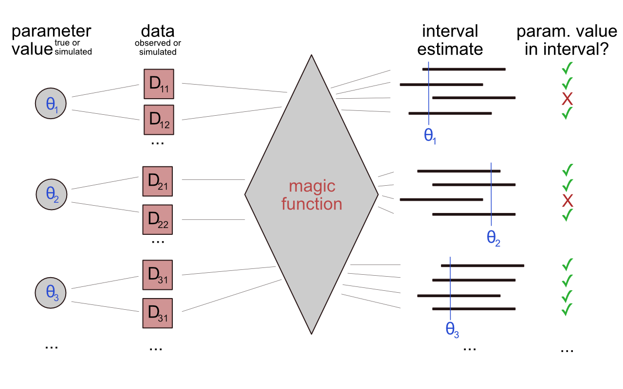
Figure 16.9: Schematic representation of what a confidence interval does: think of it as a magic function that returns intervals that contain the true value in \(\gamma\) percent of the cases.
In some complex cases, the frequentist analyst relies on functions \(g_{l}\) and \(g_{u}\) that are easy to compute but only approximately satisfy the condition \(P(X_l \le \theta_{\text{true}} \le X_u) = \frac{\gamma}{100}\). For example, we might use an asymptotically correct calculation, based on the observation that, if \(n\) grows to infinity, the binomial distribution approximates a normal distribution. We can then calculate a confidence interval as if our binomial distribution actually was a normal distribution. If \(n\) is not large enough, this will be increasingly imprecise. Rules of thumb are used to decide how big \(n\) has to be to involve at best a tolerable amount of imprecision (see the Info Box below).
For our running example (\(k = 7\), \(n=24\)), the rule of thumb mentioned in the Info Box below recommends not using the asymptotic calculation. If we did nonetheless, we would get a confidence interval of \([0.110; 0.474]\). For the binomial distribution, also a more reliable calculation exists, which yields \([0.126; 0.511]\) for the running example. (We can use numeric simulation to explore how good/bad a particular approximate calculation is, as shown in the next section.) The more reliable construction, the so-called exact method, implemented in the function binom.confint of R package binom, revolves around the close relationship between confidence intervals and \(p\)-values. (To foreshadow a later discussion: the exact \(\gamma\%\) confidence interval is the set of all parameter values for which an exact (binomial) test does not yield a significant test result as the level of \(\alpha = 1-\frac{\gamma}{100}\).)
Asymptotic approximation of a binomial confidence interval using a normal distribution.
Let \(X\) be the random variable that determines the binomial distribution, i.e., the probability of seeing \(k\) successes in \(n\) flips. For large \(n\), \(X\) approximates a normal distribution with a mean \(\mu = n \ \theta\) and a standard deviation of \(\sigma = \sqrt{n \ \theta \ (1 - \theta)}\). The random variable \(U\):
\[U = \frac{X - \mu}{\sigma} = \frac{X - n \ \theta}{\sqrt{n \ \theta \ (1-\theta)}}\] Let \(\hat{P}\) be the random variable that captures the distribution of our maximum likelihood estimates for an observed outcome \(k\):
\[\hat{P} = \frac{X}{n}\] Since \(X = \hat{P} \ n\) we obtain:
\[U = \frac{\hat{P} \ n - n \ \theta}{\sqrt{n \ \theta \ (1-\theta)}}\] We now look at the probability that \(U\) is realized to lie in a symmetric interval \([-c,c]\), centered around zero — a probability which we require to match our confidence level:
\[P(-c \le U \le c) = \frac{\gamma}{100}\] We now expand the definition of \(U\) in terms of \(\hat{P}\), equate \(\hat{P}\) with the current best estimate \(\hat{p} = \frac{k}{n}\) based on the observed \(k\) and rearrange terms, yielding the asymptotic approximation of a binomial confidence interval:
\[\left [ \hat{p} - \frac{c}{n} \ \sqrt{n \ \hat{p} \ (1-\hat{p})} ; \ \ \hat{p} + \frac{c}{n} \ \sqrt{n \ \hat{p} \ (1-\hat{p})} \right ]\]
This approximation is conventionally considered precise enough when the following rule of thumb is met:
\[n \ \hat{p} \ (1 - \hat{p}) > 9\]
16.5.1 Relation of p-values to confidence intervals
There is a close relation between \(p\)-values and confidence intervals.84 For a two-sided test of a null hypothesis \(H_0 \colon \theta = \theta_0\), with alternative hypothesis \(H_a \colon \theta \neq \theta_0\), it holds for all possible data observations \(D\) that
\[ p(D) < \alpha \ \ \text{iff} \ \ \theta_0 \not \in \text{CI}(D) \] where \(\text{CI}(D)\) is the \((1-\alpha) \cdot 100\%\) confidence interval constructed for data \(D\).
This connection is intuitive when we think about long-term error. Decisions to reject the null hypothesis are false in exactly \((\alpha \cdot 100)\%\) of the cases when the null hypothesis is true. The definition of a confidence interval was exactly the same: the true value should lay outside a \((1-\alpha) \cdot 100\%\) confidence interval in exactly \((\alpha \cdot 100)\%\) of the cases. (Of course, this is only a vague and intuitively appealing argument based on the overall rate, not any particular case.)
Exercise 16.4: \(p\)-value, confidence interval, interpretation etc.
Suppose that we have reason to believe that a coin is biased to land heads. A hypothesis test should shed light on this belief. We toss the coin \(N = 10\) times and observe \(k = 8\) heads. We set \(\alpha = 0.05\).
- What is an appropriate null hypothesis, what is an appropriate alternative hypothesis?
- Which alternative values of \(k\) provide more extreme evidence against \(H_0\)?
Values greater than 8 (we conduct a one-sided hypothesis test).
- The 95% confidence interval ranges between 0.493 and 1.0. Based on this information, decide whether the \(p\)-value is significant or non-significant. Why?
The \(p\)-value is non-significant because the value of the null hypothesis \(H_0\): \(\theta_0 = 0.5\) is contained within the 95% CI. Hence, it is not sufficiently unlikely that the observed outcome was generated by a fair coin.
- Below is the probability mass function of the Binomial distribution (our sampling distribution). The probability of obtaining exactly \(k\) successes in \(N\) independent trials is defined as: \[P(X = k)=\binom{N}{k}p^k(1-p)^{N-k},\] where \(\binom{N}{k}=\frac{N!}{k!(N-k)!}\) is the Binomial coefficient. Given the formula above, calculate the \(p\)-value (by hand) associated with our test statistic \(k\), under the assumption that \(H_0\) is true.
As this is a one-sided test, we look at those values of \(k\) that provide more extreme evidence against \(H_0\). We therefore compute the probability of at least 8 heads, given that \(H_0\) is true: \[ P(X\geq8)=P(X=8)+P(X=9)+P(X=10)\\ P(X=8)=\binom{10}{8}0.5^8(1-0.5)^{10-8}=45\cdot0.5^{10}\\ P(X=9)=\binom{10}{9}0.5^9(1-0.5)^{10-9}=10\cdot0.5^{10}\\ P(X=10)=\binom{10}{10}0.5^{10}(1-0.5)^{10-10}=1\cdot0.5^{10}\\ P(X\geq8)=0.5^{10}(45+10+1)\approx 0.0547 \]
- Based on your result in d., decide whether we should reject the null hypothesis.
As we have a non-significant \(p\)-value (\(p>\alpha\)), we fail to reject the null hypothesis. Hence, we do not have evidence in favor of the hypothesis that the coin is biased to land heads.
- Use R’s built-in function for a Binomial test to check your results.
binom.test(
  x = 8, # observed successes
  n = 10, # total no. of observations
  p = 0.5, # null hypothesis
  alternative = "greater" # alternative hypothesis
)
##
## Exact binomial test
##
## data: 8 and 10
## number of successes = 8, number of trials = 10, p-value = 0.05469
## alternative hypothesis: true probability of success is greater than 0.5
## 95 percent confidence interval:
## 0.4930987 1.0000000
## sample estimates:
## probability of success
## 0.8- The \(p\)-value is affected by the sample size \(N\). Try out different values for \(N\) while keeping the proportion of successes constant to 80%. What do you notice with regard to the \(p\)-value?
With a larger sample size, the \(p\)-value is smaller compared to 10 coin flips. It requires only a few more samples to cross the significance threshold, allowing us to reject \(H_0\). However, this is just the case if the null hypothesis is in fact false. NB: Don’t collect more data after you observed the \(p\)-value! The sample size should be fixed prior to data collection and not increased afterwards.
An important caveat applies here. There can be different (approximate) ways of defining \(p\)-values and confidence intervals. The relation described here does not hold when the (approximate) way of computing the \(p\)-value does not match the (approximate) way of computing the confidence interval.↩︎