D.2 Simon Task
![]()
The Simon task is a well-established experimental paradigm designed to study how different properties of a stimulus might interfere during information processing or decision making.
Concretely, the original Simon investigates if responses are faster and more accurate when the stimulus to respond to occurs in the same relative location (e.g., right on the screen) as the response button required by that stimulus (e.g., pressing the button p on the keyboard).
D.2.1 Experiment
You can try out the experiment for yourself here.
D.2.1.1 Participants
A total of 213 participants took part in an online version of a Simon task. Participants were students of Cognitive Science at the University of Osnabrück, taking part in courses “Introduction to Cognitive (Neuro-)Psychology” or “Experimental Psychology Lab Practice” in the summer term of 2019.
D.2.1.2 Materials & Design
Each trial started by showing a fixation cross for 200 ms in the center of the screen. Then, one of two geometrical shapes was shown for 500 ms. The target shape was either a blue square or a blue circle. The target shape appeared either on the left or right of the screen. Each trial determined uniformly at random which shape (square or circle) to show as target and where on the screen to display it (left or right). Participants were instructed to press keys q (left of keyboard) or p (right of keyboard) to identify the kind of shape on the screen. The shape-key allocation happened initially, uniformly at random once for each participant and remained constant throughout the experiment. For example, a participant may have been asked to press q for square and p for circle.
Trials were categorized as either ‘congruent’ or ‘incongruent’. They were congruent if the location of the stimulus was the same relative location as the response key (e.g., square on the right of the screen, and p key to be pressed for square) and incongruent if the stimulus was not in the same relative location as the response key (e.g., square on the right and q key to be pressed for square).
In each trial, if no key was pressed within 3 seconds after the appearance of the target shape, a message to please respond faster was displayed on the screen.
D.2.1.3 Procedure
Participants were first welcomed and made familiar with the experiment. They were told to optimize both speed and accuracy. They then practiced the task for 20 trials before starting the main task, which consisted of 100 trials. Finally, the experiment ended with a post-test survey in which participants were asked for their student IDs and the class they were enrolled in. They were also able to leave any optional comments.
D.2.2 Hypotheses
We are interested in the following hypotheses:
D.2.2.1 Hypothesis 1: Reaction times
If stimulus location interferes with information processing, we expect that it should take longer to make correct responses in the incongruent condition than in the congruent condition. Schematically, our first hypothesis about decision speed is therefore:
\[ \text{RT}_{\text{correct},\ \text{congruent}} < \text{RT}_{\text{correct},\ \text{incongruent}} \]
D.2.2.2 Hypothesis 2: Accuracy
If stimulus location interferes with information processing, we also expect to see more errors in the incongruent condition than in the congruent condition. Schematically, our second hypothesis about decision accuracy is therefore:
\[ \text{Accuracy}_{\text{correct},\ \text{congruent}} > \text{Accuracy}_{\text{correct},\ \text{incongruent}} \]
D.2.3 Results
D.2.3.1 Loading and inspecting the data
We load the data and show a summary of the variables stored in the tibble:
d <- aida::data_ST_raw
glimpse(d)
## Rows: 25,560
## Columns: 15
## $ submission_id <dbl> 7432, 7432, 7432, 7432, 7432, 7432, 7432, 7432, 7432, …
## $ RT <dbl> 1239, 938, 744, 528, 706, 547, 591, 652, 627, 485, 515…
## $ condition <chr> "incongruent", "incongruent", "incongruent", "incongru…
## $ correctness <chr> "correct", "correct", "correct", "correct", "correct",…
## $ class <chr> "Intro Cogn. Neuro-Psychology", "Intro Cogn. Neuro-Psy…
## $ experiment_id <dbl> 52, 52, 52, 52, 52, 52, 52, 52, 52, 52, 52, 52, 52, 52…
## $ key_pressed <chr> "q", "q", "q", "q", "p", "p", "q", "p", "q", "q", "q",…
## $ p <chr> "circle", "circle", "circle", "circle", "circle", "cir…
## $ pause <dbl> 1896, 1289, 1705, 2115, 2446, 2289, 2057, 2513, 1865, …
## $ q <chr> "square", "square", "square", "square", "square", "squ…
## $ target_object <chr> "square", "square", "square", "square", "circle", "cir…
## $ target_position <chr> "right", "right", "right", "right", "left", "right", "…
## $ timeSpent <dbl> 7.565417, 7.565417, 7.565417, 7.565417, 7.565417, 7.56…
## $ trial_number <dbl> 1, 2, 3, 4, 5, 6, 7, 8, 9, 10, 11, 12, 13, 14, 15, 16,…
## $ trial_type <chr> "practice", "practice", "practice", "practice", "pract…The most important columns in this data set for our purposes are:
submission_id: an ID identifying each participantRT: the reaction time for each trialcondition: whether the trial was a congruent or an incongruent trialcorrectness: whether the answer in the current trial was correct or incorrecttrial_type: whether the data is from a practice or a main test trial
D.2.3.2 Cleaning the data
We look at outlier-y behavior at the level of individual participants first, then at the level of individual trials.
D.2.3.2.1 Individual-level error rates & reaction times
It is conceivable that some participants did not take the task seriously. They may have just fooled around. We will therefore inspect each individual’s response patterns and reaction times. If participants appear to have “misbehaved”, we discard all of their data. (CAVEAT: Notice the researcher degrees of freedom in the decision of what counts as “misbehavior”! It is therefore that choices like these are best committed to in advance, e.g., via pre-registration!)
We can calculate the mean reaction times and the error rates for each participant.
d_individual_summary <- d %>%
  filter(trial_type == "main") %>%    # look at only data from main trials
  group_by(submission_id) %>%         # calculate the following for each individual
  summarize(mean_RT = mean(RT),
            error_rate = 1 - mean(ifelse(correctness == "correct", 1, 0)))
head(d_individual_summary)
## # A tibble: 6 × 3
## submission_id mean_RT error_rate
## <dbl> <dbl> <dbl>
## 1 7432 595. 0.0500
## 2 7433 458. 0.0400
## 3 7434 531. 0.0400
## 4 7435 433. 0.12
## 5 7436 748. 0.0600
## 6 7437 522. 0.12Let’s plot this summary information:
d_individual_summary %>%
  ggplot(aes(x = mean_RT, y = error_rate)) +
  geom_point()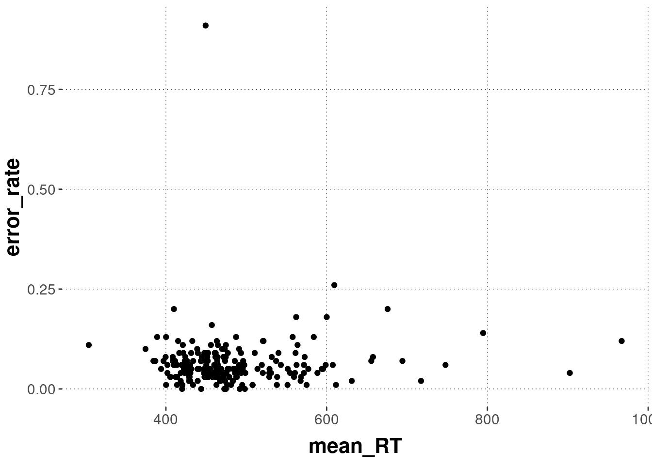
Here’s a crude way of branding outlier-participants:
d_individual_summary <- d_individual_summary %>%
  mutate(outlier = case_when(mean_RT < 350 ~ TRUE,
                             mean_RT > 750 ~ TRUE,
                             error_rate > 0.5 ~ TRUE,
                             TRUE ~ FALSE))
d_individual_summary %>%
  ggplot(aes(x = mean_RT, y = error_rate)) +
  geom_point() +
  geom_point(data = filter(d_individual_summary, outlier == TRUE),
             color = "firebrick", shape = "square", size = 5)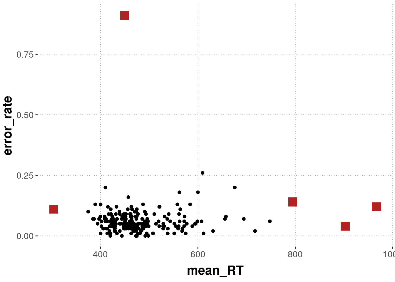
We then clean the data set in a first step by removing all participants identified as outlier-y:
d <- full_join(d, d_individual_summary, by = "submission_id") # merge the tibbles
d <- filter(d, outlier == FALSE)
message("We excluded ", sum(d_individual_summary$outlier), " participants for suspicious mean RTs and higher error rates.")
## We excluded 5 participants for suspicious mean RTs and higher error rates.D.2.3.2.2 Trial-level reaction times
It is also conceivable that individual trials resulted in early accidental key presses or were interrupted in some way or another. We therefore look at the overall distribution of RTs and determine what to exclude. (Again, it is important that decisions of what to exclude should ideally be publicly preregistered before data analysis.)
Let’s first plot the overall distribution of RTs.
d %>% ggplot(aes(x = RT)) +
  geom_histogram() +
  geom_jitter(aes(x = RT, y = 1), alpha = 0.3, height = 300)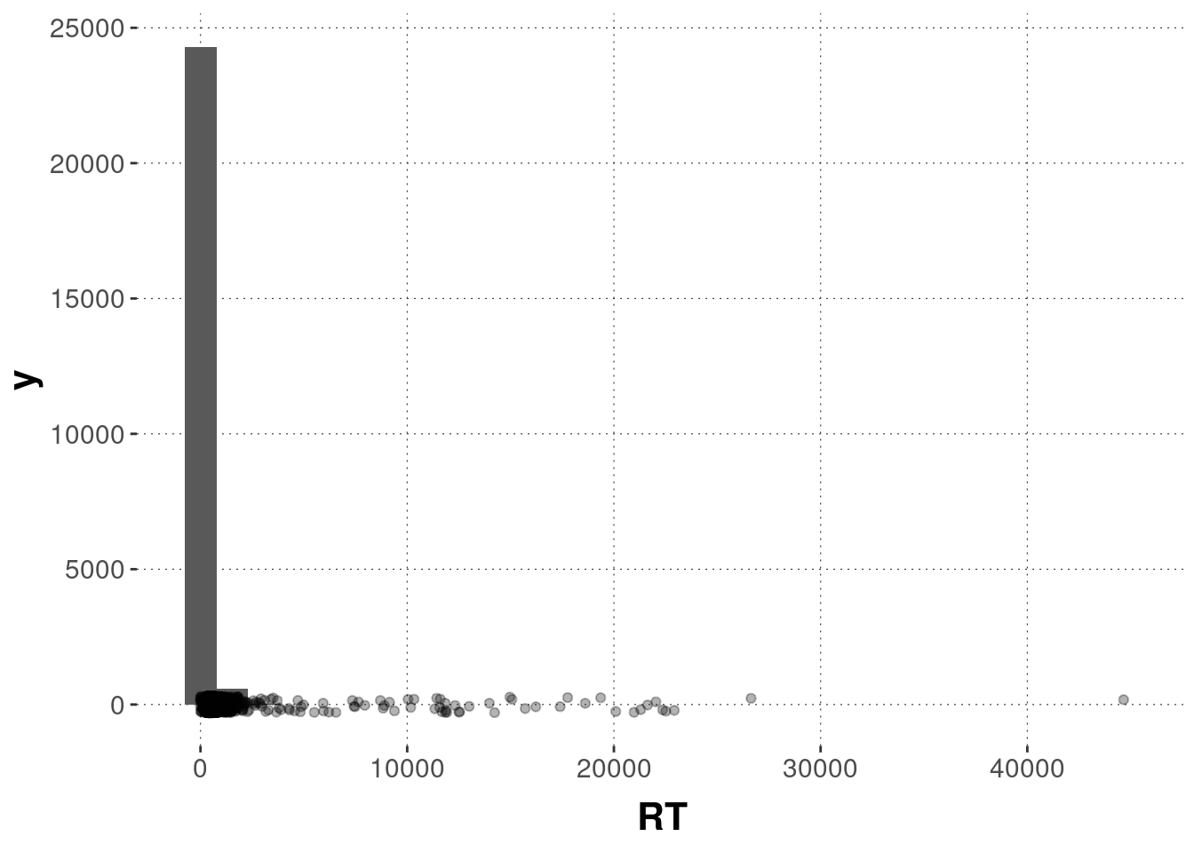
Some very long RTs make this graph rather uninformative. Let’s therefore exclude all trials that lasted longer than 1 second and also all trials with reaction times under 100 ms.
message(
  "We exclude ",
  nrow(filter(d, RT < 100)) + nrow(filter(d, RT > 1000)),
  " trials based on too fast or too slow RTs."
)
# exclude these trials
d <- filter(d, RT > 100 & RT < 1000)
Here’s the distribution of RTs after cleaning:
d %>% ggplot(aes(x = RT)) +
  geom_histogram() +
  geom_jitter(aes(x = RT, y = 1), alpha = 0.3, height = 300)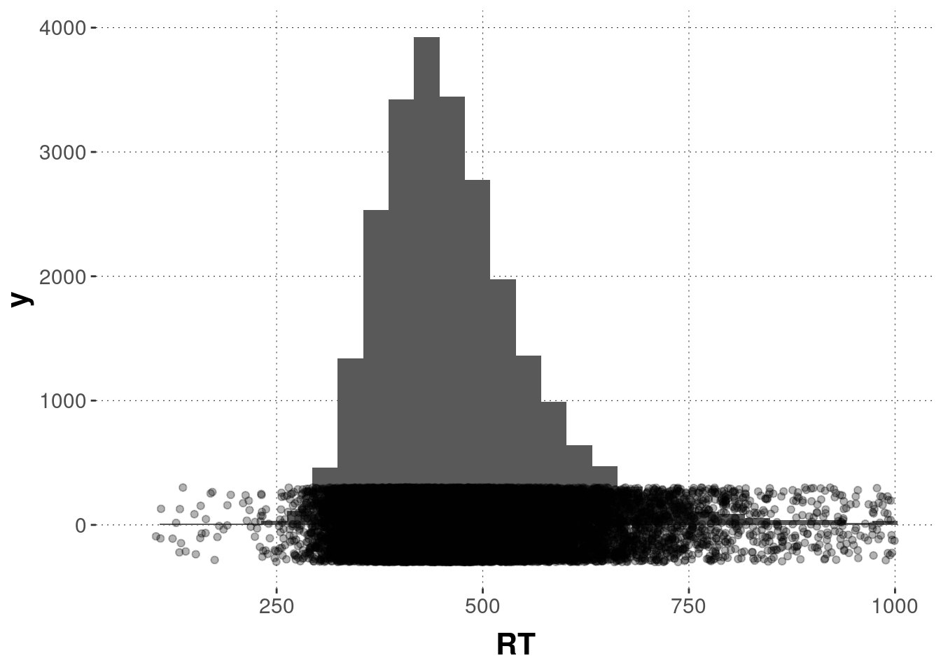
Finally, we discard the training trials:
d <- filter(d, trial_type == "main")D.2.3.3 Hypothesis-driven summary statistics
D.2.3.3.1 Hypothesis 1: Reaction times
We are mostly interested in the influence of congruency on the reaction times in the trials where participants gave a correct answer. But here we also look at, for comparison, the reaction times for incorrect trials.
Here is a summary of the means and standard deviations for each condition:
d_sum <- d %>%
  group_by(correctness, condition) %>%
  summarize(mean_RT = mean(RT),
            sd_RT = sd(RT))
d_sum
## # A tibble: 4 × 4
## # Groups: correctness [2]
## correctness condition mean_RT sd_RT
## <chr> <chr> <dbl> <dbl>
## 1 correct congruent 453. 99.6
## 2 correct incongruent 477. 85.1
## 3 incorrect congruent 462 97.6
## 4 incorrect incongruent 393. 78.1Numerically, the reaction times for the correct-congruent trials are indeed faster than for the correct-incongruent trials.
Here’s a plot of the reaction times split up by whether the answer was correct and whether the trial was congruent or incongruent.
d %>% ggplot(aes(x = RT)) +
  geom_jitter(aes(y = 0.0005), alpha = 0.1, height = 0.0005) +
  geom_density(fill = "gray", alpha = 0.5) +
  geom_vline(data = d_sum,
             mapping = aes(xintercept = mean_RT),
             color = "firebrick") +
  facet_grid(condition ~ correctness)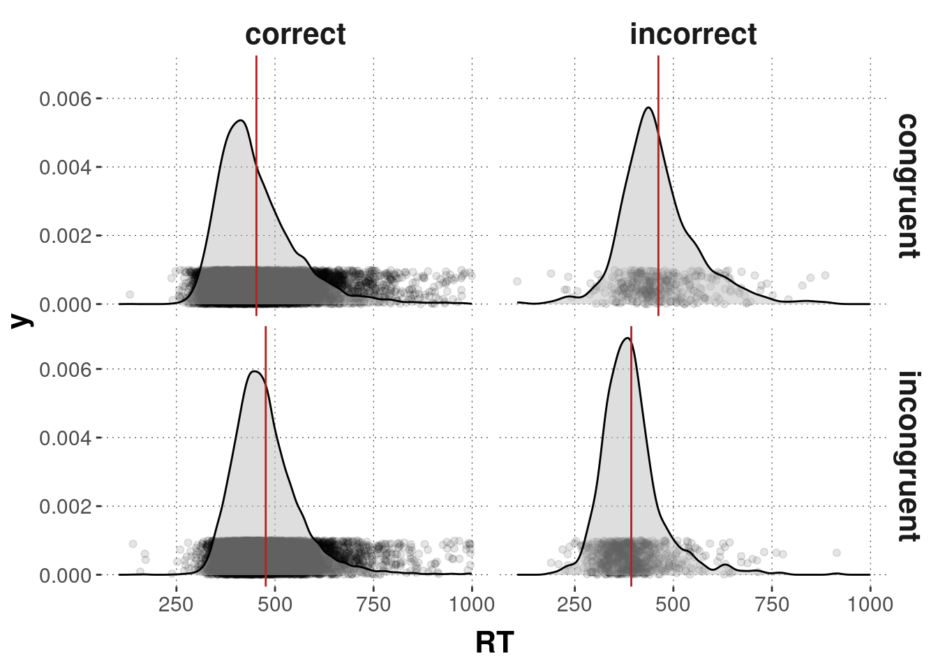
D.2.3.3.2 Hypothesis 2: Accuracy
Our second hypothesis is about the proportion of correct answers, comparing the congruent against the incongruent trials. Here is a summary statistic for the acurracy in both conditions:
d %>% group_by(condition) %>%
  summarize(acurracy = mean(correctness == "correct"))
## # A tibble: 2 × 2
## condition acurracy
## <chr> <dbl>
## 1 congruent 0.961
## 2 incongruent 0.923Again, numerically it seems that the hypothesis is borne out that accuracy is higher in the congruent trials.