13.2 Extracting posterior samples

The function brms::posterior_samples extracts the samples from the posterior which are part of the brmsfit object.⁶⁰

post_samples_temperature <- brms::posterior_samples(fit_temperature)  %>% select(-lp__,-lprior)
head(post_samples_temperature)

##   b_Intercept      b_year     sigma
## 1   -4.328078 0.006692733 0.4100904
## 2   -4.202760 0.006633079 0.4050540
## 3   -2.887432 0.005926658 0.4006999
## 4   -4.580320 0.006821945 0.3996143
## 5   -2.587499 0.005782539 0.3916289
## 6   -4.247891 0.006654168 0.4081150

These extracted samples can be used as before, e.g., to compute our own summary tibble:

map_dfr(post_samples_temperature, aida::summarize_sample_vector) %>% 
  mutate(Parameter = colnames(post_samples_temperature[1:3]))

## # A tibble: 3 × 4
##   Parameter     `|95%`     mean   `95%|`
##   <chr>          <dbl>    <dbl>    <dbl>
## 1 b_Intercept -4.69    -3.51    -2.32   
## 2 b_year       0.00563  0.00627  0.00689
## 3 sigma        0.373    0.405    0.440

Or for manual plotting:⁶¹

post_samples_temperature %>% 
  pivot_longer(cols = everything()) %>% 
  ggplot(aes(x = value)) +
  geom_density() +
  facet_wrap(~name, scales = "free")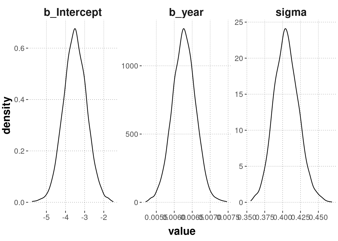

---

60. The column lp__ gives the log probability of the data for the corresponding parameter values in each row. This is useful information for model checking and model comparison, but we will neglect it here.↩︎

61. There are also specialized packages for plotting the output of Stan models and brms model fits, such as the excellent tidybayes and ggdist packages.↩︎