11.2 Data and models for this chapter

This chapter uses two case studies as running examples: the (fictitious) 24/7 coin-flip example analyzed with the Binomial model, and data from the Simon task analyzed with a so-called Bayesian $t$-test model.

11.2.1 24/7

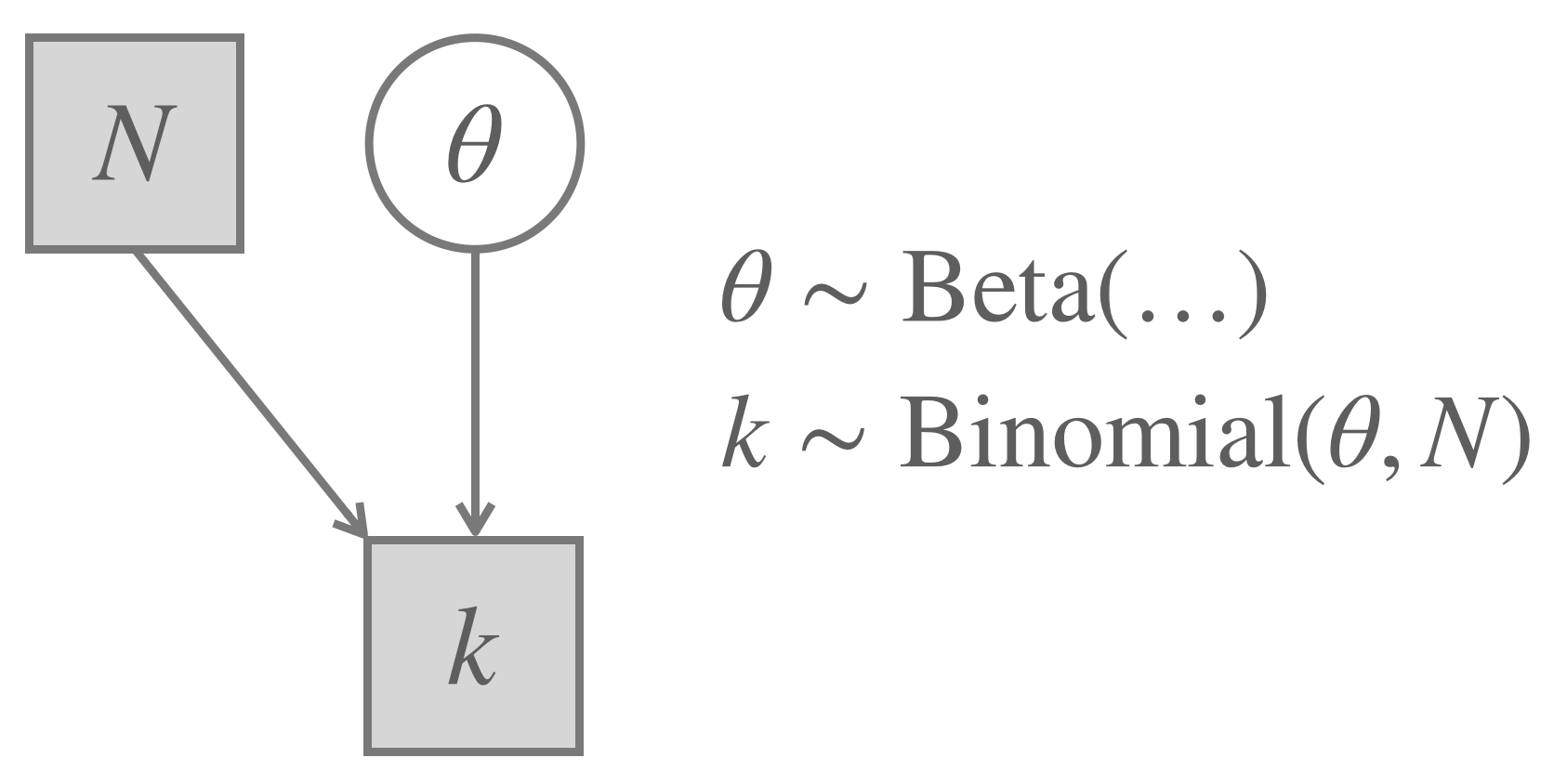
We will use the same (old) example of binomial data: $k = 7$ heads out of $N = 24$ coin flips. Just as before, we will use the standard binomial model with a flat Beta prior, shown below in graphical notation:

Figure 11.2: The Binomial Model (repeated from before).

We are interested in the following hypotheses:

Point-valued: $\theta_c = 0.5$
ROPE-d $\theta_c = \in [0.5 - \epsilon; 0.5 + \epsilon]$ with $\epsilon = 0.01$
Directional $\theta_c < 0.5$

11.2.2 Simon task

The Simon task is a classic experimental design to investigate interference of, intuitively put, task-relevant properties and task-irrelevant properties. Chapter D.2 introduces the experiment and the (cleaned) data we analyze here.

data_simon_cleaned <- aida::data_ST

The most important columns in this data set for our current purposes are:

RT: The reaction time for each trial.
condition: Whether the trial was a congruent or an incongruent trial.

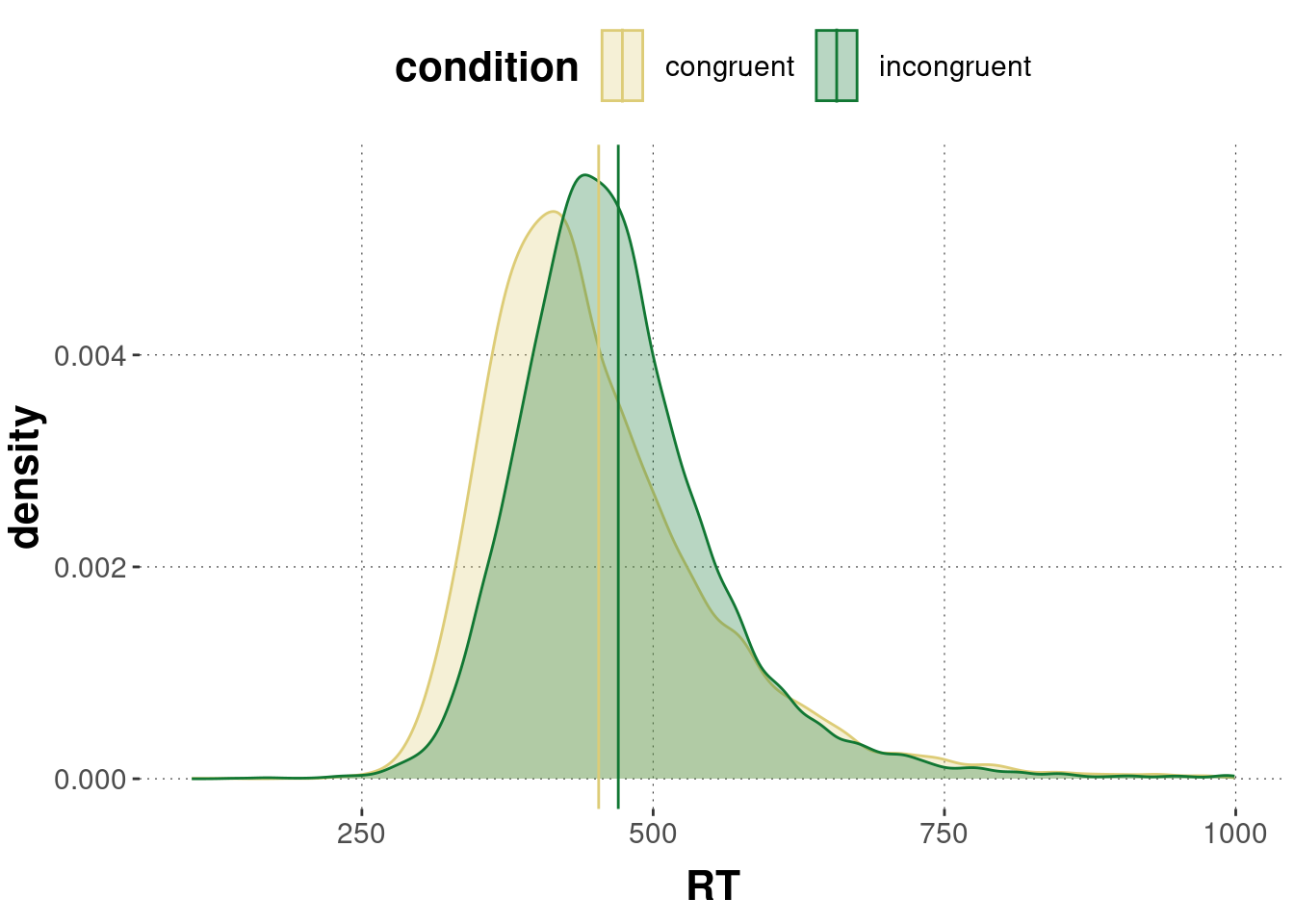
Concretely, we are interested in comparing the mean reaction times across conditions:

Distribution of reaction times of correct answers in the congruent and incongruent condition of the Simon task. Vertical lines indicate the mean of each condition.

Figure 11.3: Distribution of reaction times of correct answers in the congruent and incongruent condition of the Simon task. Vertical lines indicate the mean of each condition.

In order to compare the means of continuous measurements between two groups we will use a so-called $t$-test model. (The reason why this is called a “$t$-test model” is historical and will become clear in Chapter 16.) There are different variations of Bayesian $t$-test models. Here, we use the one proposed by Gönen et al. (2005), which enables us to compute Bayes factor model comparison for point-valued hypotheses analytically. The model is shown in Figure 11.4.

Bayesian $t$-test model following Gönen et al. [-@GoenenJohnson2005] for inferences about the difference in means in the Simon task data.

Figure 11.4: Bayesian $t$-test model following Gönen et al. (2005) for inferences about the difference in means in the Simon task data.

The model in Figure 11.4 assumes that there are two vectors $y_1$ and $y_2$ of continuous measurements. In our case, these are the continuous measurements of reaction times in the incongruent ($y_1$) and congruent ($y_2$) group. The model further assumes that all measurements in $y_1$ and $y_2$ are samples from two normal distributions, one for each group, with shared variance but possibly different means. The means of the two normal distributions are represented in terms of the midpoint $\mu$ between the means of either group. The model is set-up in such a way that there is a difference parameter $\delta$ which specifies the standardized difference between group means. Standardization here means that the difference between the means is represented in relation to the variance of the measurements in each group (which is assumed to be the same in both groups). The free variables in this model are therefore: the average of the group means $\mu$, the standardized difference $\delta$ of the group means from each other, and the common variance $\sigma$ of measurements in each group. The priors for these parameters are chosen in such a way as to enable direct calculation of Bayes factors for point-valued hypotheses. Notice that, by explicitly representing the difference parameter $\delta$ in the model, it is possible to put different kinds of a priori assumptions about the likely differences between groups directly into the model, namely in the form of $\mu_g$ and $g$, which are not free model parameters, but will be set by us modelers, here as $\mu_g = 0$ and $g = 1$.

We focus on the first hypothesis spelled out in Chapter D.2, namely that the correct choices are faster in the congruent condition than in the incongruent condition. So, based on this data and model, we are interested in the following statistical hypotheses:

Point-valued: $\delta = 0$
ROPE-d $\delta = \in [0 - \epsilon; 0 + \epsilon]$ with $\epsilon = 0.1$
Directional $\delta > 0$

Exercise 11.1

Paraphrase the three hypotheses given for the 24/7 data and the three hypotheses given for the Simon task in your own words.

24/7:

Point-valued: $\theta_c = 0.5$ - the coin is fair, with a bias of exactly 0.5
ROPE-d $\theta_c = \in [0.5 - \epsilon; 0.5 + \epsilon]$ with $\epsilon = 0.01$ - the coins bias lies between 0.49 and 0.51
Directional $\theta_c < 0.5$ - the coin is biased towards tails

Simon task:

Point-valued: $\delta = 0$ - the difference between the means of reaction times in both groups is 0
ROPE-d $\delta = \in [0 - \epsilon; 0 + \epsilon]$ with $\epsilon = 0.1$ - the absolute difference between the means of reaction times in both groups is no bigger than 10% of the variance in both groups
Directional $\delta > 0$ - the mean reaction time in group 1 is bigger than the mean reaction time in group 2

References

Mithat Gonen, Yonggang Lu & Peter H. Westfall, Wesley O. Johnson. 2005. “The Bayesian Two-Sample t-Test.” The American Statistician 59 (3): 252–57. https://doi.org/10.1198/000313005X55233.