\(P(\text{miss}) = P(\text{miss, rainy}) + P(\text{miss, dry}) = 0.6 + 0.1 = 0.7\)
7.2 Structured events & marginal distributions
The single urn scenario of the last section is a very basic first example. To pave the way for learning about conditional probability and Bayes rule in the next sections, let us consider a slightly more complex example. We call it the flip-and-draw scenario.
7.2.1 Probability table for a flip-and-draw scenario
Suppose we have two urns. Both have \(N=10\) balls. Urn 1 has \(k_1=2\) black and \(N-k_1 = 8\) white balls. Urn 2 has \(k_2=4\) black and \(N-k_2=6\) white balls. We sometimes draw from urn 1, sometimes from urn 2. To decide from which urn a ball should be drawn, we flip a fair coin. If it comes up heads, we draw from urn 1; if it comes up tails, we draw from urn 2. The process is visualized in Figure 7.2 below.
An elementary outcome of this two-step process of flip-and-draw is a pair \(\langle \text{outcome-flip}, \text{outcome-draw} \rangle\). The set of all possible such outcomes is:
\[\Omega_{\text{flip-and-draw}} = \left \{ \langle \text{heads}, \text{black} \rangle, \langle \text{heads}, \text{white} \rangle, \langle \text{tails}, \text{black} \rangle, \langle \text{tails}, \text{white} \rangle \right \}\,.\]
The probability of event \(\langle \text{heads}, \text{black} \rangle\) is given by multiplying the probability of seeing “heads” on the first flip, which happens with probability \(0.5\), and then drawing a black ball, which happens with probability \(0.2\), so that \(P(\langle \text{heads}, \text{black} \rangle) = 0.5 \times 0.2 = 0.1\). The probability distribution over \(\Omega_{\text{flip-draw}}\) is consequently as in Table 7.1. (If in doubt, start flipping & drawing and count your outcomes or use the WebPPL code box in the exercise below to simulate flips-and-draws.)
| heads | tails | |
|---|---|---|
| black | \(0.5 \times 0.2 = 0.1\) | \(0.5 \times 0.4 = 0.2\) |
| white | \(0.5 \times 0.8 = 0.4\) | \(0.5 \times 0.6 = 0.3\) |
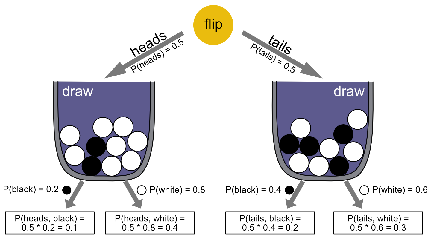
Figure 7.2: The flip-and-draw scenario, with transition and full path probabilities.
7.2.2 Structured events and joint-probability distributions
Table 7.1 is an example of a joint probability distribution over a structured event space, which here has two dimensions. Since our space of outcomes is the Cartesian product of two simpler outcome spaces, namely \(\Omega_{flip\text{-}\&\text{-}draw} = \Omega_{flip} \times \Omega_{draw}\),36 we can use notation \(P(\text{heads}, \text{black})\) as shorthand for \(P(\langle \text{heads}, \text{black} \rangle)\). More generally, if \(\Omega = \Omega_1 \times \dots \Omega_n\), we can think of \(P \in \Delta(\Omega)\) as a joint probability distribution over \(n\) subspaces.
7.2.3 Marginalization
If \(P\) is a joint probability distribution over event space \(\Omega = \Omega_1 \times \dots \Omega_n\), the marginal distribution over subspace \(\Omega_i\), \(1 \le i \le n\) is the probability distribution that assigns to all \(A_i \subseteq \Omega_i\) the probability (where notation \(P(\dots, \omega, \dots )\) is shorthand for \(P(\dots, \{\omega \}, \dots)\)):37
\[ \begin{align*} P(A_i) & = \sum_{\omega_1 \in \Omega_{1}} \sum_{\omega_2 \in \Omega_{2}} \dots \sum_{\omega_{i-1} \in \Omega_{i-1}} \sum_{\omega_{i+1} \in \Omega_{i+1}} \dots \sum_{\omega_n \in \Omega_n} P(\omega_1, \dots, \omega_{i-1}, A_{i}, \omega_{i+1}, \dots \omega_n) \end{align*} \]
For example, the marginal distribution of draws derivable from Table 7.1 has \(P(\text{black}) = P(\text{heads, black}) + P(\text{tails, black}) = 0.3\) and \(P(\text{white}) = 0.7\).38 The marginal distribution of coin flips derivable from the joint probability distribution in Table 7.1 gives \(P(\text{heads}) = P(\text{tails}) = 0.5\), since the sum of each column is exactly \(0.5\).
Exercise 7.3
- Given the following joint probability table, compute the probability that a student does not attend the lecture, i.e., \(P(\text{miss})\).
| attend | miss | |
|---|---|---|
| rainy | 0.1 | 0.6 |
| dry | 0.2 | 0.1 |
- Play around with the following WebPPL implementation of the flip-and-draw scenario. Change the ‘input values’ of the coin’s bias and the probabilities of sampling a black ball from either urn. Inspect the resulting joint probability tables and the marginal distribution of observing “black”. Try to find at least three different parameter settings that result in the marginal probability of black being 0.7.
// you can play around with the values of these variables
var coin_bias = 0.5          // coin bias
var prob_black_urn_1 = 0.2   // probability of drawing "black" from urn 1
var prob_black_urn_2 = 0.4   // probability of drawing "black" from urn 2

///fold:
// convenience function for showing nicer tables
var condProb2Table = function(condProbFct, row_names, col_names, precision){
  var matrix = map(function(row) {
    map(function(col) {
      _.round(Math.exp(condProbFct.score({"coin": row, "ball": col})),precision)},
        col_names)},
                   row_names)
  var max_length_col = _.max(map(function(c) {c.length}, col_names))
  var max_length_row = _.max(map(function(r) {r.length}, row_names))
  var header = _.repeat(" ", max_length_row + 2)+ col_names.join("  ") + "\n"
  var row = mapIndexed(function(i,r) { _.padEnd(r, max_length_row, " ") + "  " +
                       mapIndexed(function(j,c) {
                          _.padEnd(matrix[i][j], c.length+2," ")},
                                  col_names).join("") + "\n" },
                           row_names).join("")
  return header + row
}
// flip-and-draw scenario model
var model = function() {
  var coin_flip = flip(coin_bias)  == 1 ? "heads" : "tails"
  var prob_black_selected_urn = coin_flip == "heads" ?
    prob_black_urn_1 : prob_black_urn_2
  var ball_color = flip(prob_black_selected_urn) == 1 ? "black" : "white"
  return({coin: coin_flip, ball: ball_color})
}
// infer model and display as (custom-made) table
var inferred_model = Infer({method: 'enumerate'}, model)
display("Joint probability table")
display(condProb2Table(inferred_model, ["tails", "heads"], ["white", "black"], 3))
display("\nMarginal probability of ball color")
viz(marginalize(inferred_model, function(x) {return x.ball}))
///
Three possibilities for obtaining a value of 0.7 for the marginal probability of “black”:
prob_black_urn_1 = prob_black_urn_2 = 0.7coin_bias = 1andprob_black_urn_1 = 0.7coin_bias = 0.5,prob_black_urn_1 = 0.8andprob_black_urn_2 = 0.6
With \(\Omega_{\text{flip}} = \left \{ \text{heads}, \text{tails} \right \}\) and \(\Omega_{\text{draw}} = \left \{ \text{black}, \text{white} \right \}\).↩︎
This notation, using \(\sum\), assumes that subspaces are countable. In other cases, a parallel definition with integrals can be used.↩︎
The term “marginal distribution” derives from such probability tables, where traditionally the sum of each row/column was written in the margins.↩︎