name: nominal variableage: metric variablegender: nominal variablehandedness: binary variableheight: metric variableeducation: ordinal variablehas_pets: Boolean variablemood: ordinal variable
3.3 On the notion of “variables”
Data used for data analysis, even if it is “raw data”, i.e., data before preprocessing and cleaning, is usually structured or labeled in some way or other. Even if the whole data we have is a vector of numbers, we would usually know what these numbers represent. For instance, we might just have a quintuple of numbers, but we would (usually/ideally) know that these represent the results of an IQ test.
# a simple data vector of IQ-scores
IQ_scores <- c(102, 115, 97, 126, 87)
Or we might have a Boolean vector with the information of whether each of five students passed an exam. But even then we would (usually/ideally) know the association between names and test results, as in a table like this:
# who passed the exam
exam_results <-
  tribble(
    ~student,   ~pass,
    "Jax",      TRUE,
    "Jason",    FALSE,
    "Jamie",    TRUE
  )
Association of information, as between different columns in a table like the one above, is crucial. Most often, we have more than one kind of observation that we care about. Most often, we care about systematic relationships between different observables in the world. For instance, we might want to look at a relation between, on the one hand, the chance of passing an exam and, on the other hand, the proportion of attendance of the course’s tutorial sessions:
# proportion of tutorials attended and exam pass/fail
exam_results <-
  tribble(
    ~student,   ~tutorial_proportion,   ~pass,
    "Jax",      0.0,                    TRUE,
    "Jason",    0.78,                   FALSE,
    "Jamie",    0.39,                   TRUE
  )
exam_results
## # A tibble: 3 × 3
## student tutorial_proportion pass
## <chr> <dbl> <lgl>
## 1 Jax 0 TRUE
## 2 Jason 0.78 FALSE
## 3 Jamie 0.39 TRUEData of this kind is also called rectangular data, i.e., data that fits into a rectangular table (More on the structure of rectangular data in Section 4.2.). In the example above, every column represents a variable of interest. A (data) variable stores the observations that are of the same kind.15
Different kinds of variables are distinguished based on the structural properties of the kinds of observations that they represent. Common types of variables are, for instance:
- nominal variable: each observation is an instance of a (finite) set of clearly distinct categories, lacking a natural ordering;
- binary variable: special case of a nominal variable where there are only two categories;
- Boolean variable: special case of a binary variable where the two categories are Boolean values “true” and “false”;
- ordinal variable: each observation is an instance of a (finite) set of clearly distinct and naturally ordered categories, but there is no natural meaning of distance between categories (i.e., it makes sense to say that A is “more” than B but not that A is three times “more” than B);
- metric variable: each observation is isomorphic to a subset of the reals and interval-scaled (i.e., it makes sense to say that A is three times “more” than B);
Examples of some different kinds of variables are shown in Figure 3.2, and Table 3.2 lists common and/or natural ways of representing different kinds of (data) variables in R.
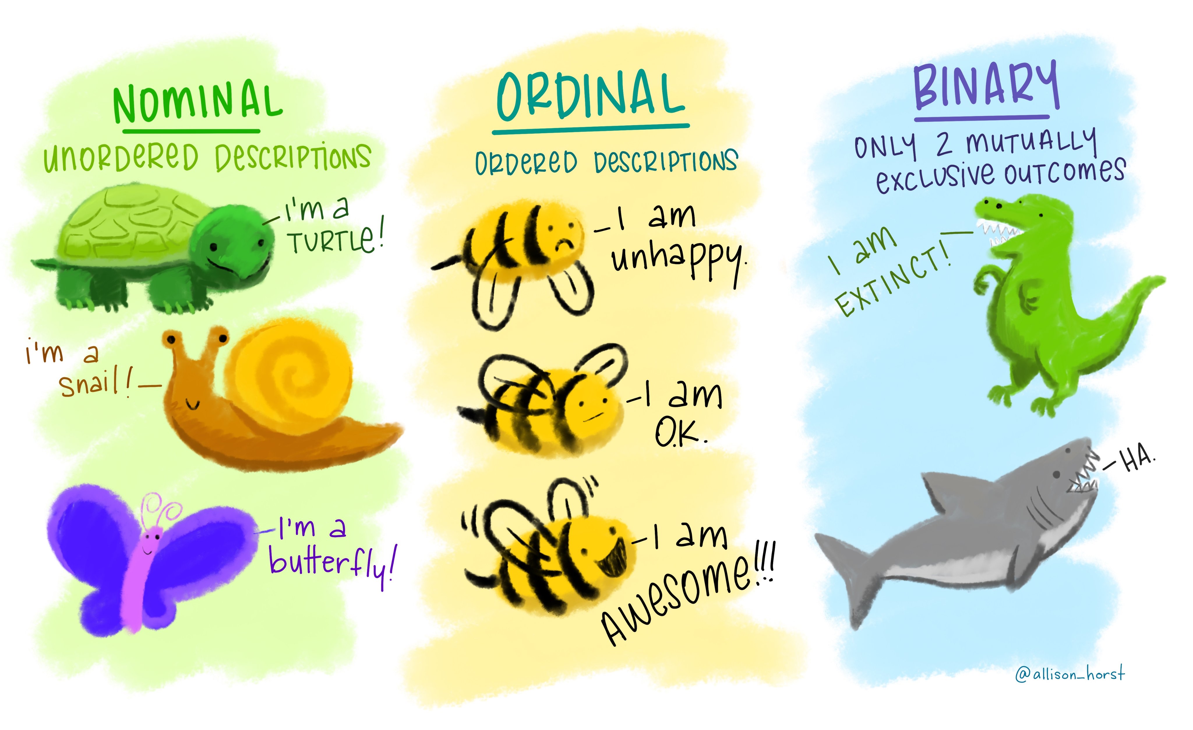
Figure 3.2: Examples of different kinds of (data) variables. Artwork by allison_horst.
| variable type | representation in R |
|---|---|
| nominal / binary | unordered factor |
| Boolean | logical vector |
| ordinal | ordered factor |
| metric | numeric vector |
In experimental data, we also distinguish the dependent variable(s) from the independent variable(s). The dependent variables are the variables that we do not control or manipulate in the experiment, but the ones that we are curious to record (e.g., whether a patient recovered from an illness within a week). Dependent variables are also called to-be-explained variables. The independent variables are the variables in the experiment that we manipulate (e.g., which drug to administer), usually with the intention of seeing a particular effect on the dependent variables. Independent variables are also called explanatory variables.
Exercise 3.1: Variables
You are given the following table of observational data:
## # A tibble: 7 × 8
##   name    age gender     handedness height education     has_pets mood
##   <chr> <dbl> <chr>      <chr>       <dbl> <chr>         <lgl>    <chr>
## 1 A        24 female     right        1.74 undergraduate FALSE    neutral
## 2 B        32 non-binary right        1.68 graduate      TRUE     happy
## 3 C        23 male       left         1.62 high school   TRUE     OK
## 4 D        27 male       right        1.84 graduate      FALSE    very happy
## 5 E        26 non-binary left         1.59 undergraduate FALSE    very happy
## 6 F        28 female     right        1.66 graduate      TRUE     OK
## 7 G        35 male       right        1.68 high school   FALSE    neutral
For each column, decide which type of variable (nominal, binary, etc.) is stored.