5.1 Counts and proportions
![]()
Very familiar instances of summary statistics are counts and frequencies. While there is no conceptual difficulty in understanding these numerical measures, we have yet to see how to obtain counts for categorical data in R. The Bio-Logic Jazz-Metal data set provides nice material for doing so. If you are unfamiliar with the data and the experiment that generated it, please have a look at Appendix Chapter D.4.
5.1.1 Loading and inspecting the data
We load the preprocessed data immediately (see Appendix D.4 for details on how this preprocessing was performed).
data_BLJM_processed <- aida::data_BLJMThe preprocessed data lists, for each participant (in column submission_id) the binary choice (in column response) in a particular condition (in column condition).
head(data_BLJM_processed)## # A tibble: 6 × 3
## submission_id condition response
## <dbl> <chr> <chr>
## 1 379 BM Beach
## 2 379 LB Logic
## 3 379 JM Metal
## 4 378 JM Metal
## 5 378 LB Logic
## 6 378 BM Beach5.1.2 Obtaining counts with n, count and tally
To obtain counts, the dplyr package offers the functions n, count and tally, among others.20 The function n does not take arguments and is useful for counting rows. It works inside of summarise and mutate and is usually applied to grouped data sets. For example, we can get a count of how many observations the data in data_BLJM_processed contains for each condition by first grouping by variable condition and then calling n (without arguments) inside of summarise:
data_BLJM_processed %>%
  group_by(condition) %>%
  summarise(nr_observation_per_condition = n()) %>%
  ungroup()
## # A tibble: 3 × 2
## condition nr_observation_per_condition
## <chr> <int>
## 1 BM 102
## 2 JM 102
## 3 LB 102Notice that calling n without grouping just gives you the number of rows in the data set:
data_BLJM_processed %>%
  summarize(n_rows = n())
## # A tibble: 1 × 1
## n_rows
## <int>
## 1 306This can also be obtained simply by (although in a different output format!):
nrow(data_BLJM_processed)## [1] 306Counting can be helpful also when getting acquainted with a data set, or when checking whether the data is complete. For example, we can verify that every participant in the experiment contributed three data points like so:
data_BLJM_processed %>%
  group_by(submission_id) %>%
  summarise(nr_data_points = n())
## # A tibble: 102 × 2
## submission_id nr_data_points
## <dbl> <int>
## 1 278 3
## 2 279 3
## 3 280 3
## 4 281 3
## 5 282 3
## 6 283 3
## 7 284 3
## 8 285 3
## 9 286 3
## 10 287 3
## # … with 92 more rowsThe functions tally and count are essentially just convenience wrappers around n. While tally expects that the data is already grouped in the relevant way, count takes a column specification as an argument and does the grouping (and final ungrouping) implicitly.
For instance, the following code blocks produce the same output, one using n, the other using count, namely the total number of times a particular response has been given in a particular condition:
data_BLJM_processed %>%
  group_by(condition, response) %>%
  summarise(n = n())
## # A tibble: 6 × 3
## # Groups: condition [3]
## condition response n
## <chr> <chr> <int>
## 1 BM Beach 44
## 2 BM Mountains 58
## 3 JM Jazz 64
## 4 JM Metal 38
## 5 LB Biology 58
## 6 LB Logic 44data_BLJM_processed %>%
# use function `count` from `dplyr` package
dplyr::count(condition, response)## # A tibble: 6 × 3
## condition response n
## <chr> <chr> <int>
## 1 BM Beach 44
## 2 BM Mountains 58
## 3 JM Jazz 64
## 4 JM Metal 38
## 5 LB Biology 58
## 6 LB Logic 44So, these counts suggest that there is an overall preference for mountains over beaches, Jazz over Metal and Biology over Logic. Who would have known!?
These counts are overall numbers. They do not tell us anything about any potentially interesting relationship between preferences. So, let’s have a closer look at the number of people who selected which music-subject pair. We collect these counts in variable BLJM_associated_counts. We first need to pivot the data, using pivot_wider, to make sure each participant’s choices are associated with each other, and then take the counts of interest:
BLJM_associated_counts <- data_BLJM_processed %>%
  pivot_wider(names_from = condition, values_from = response) %>%
  # drop the Beach vs. Mountain condition
  select(-BM) %>%
  dplyr::count(JM, LB)
BLJM_associated_counts
## # A tibble: 4 × 3
## JM LB n
## <chr> <chr> <int>
## 1 Jazz Biology 38
## 2 Jazz Logic 26
## 3 Metal Biology 20
## 4 Metal Logic 18We can also produce a table of proportions from this, simply by dividing the column called n by the total number of observations using sum(n). We can also flip the table around into a more convenient (though messy) representation:
BLJM_associated_counts %>%
  # look at relative frequency, not total counts
  mutate(n = n / sum(n)) %>%
  pivot_wider(names_from = LB, values_from = n)
## # A tibble: 2 × 3
## JM Biology Logic
## <chr> <dbl> <dbl>
## 1 Jazz 0.373 0.255
## 2 Metal 0.196 0.176Eye-balling this table of relative frequencies, we might indeed hypothesize that preference for musical style is not independent of preference for an academic subject. The impression is corroborated by looking at the plot in Figure 5.1. More on this later!
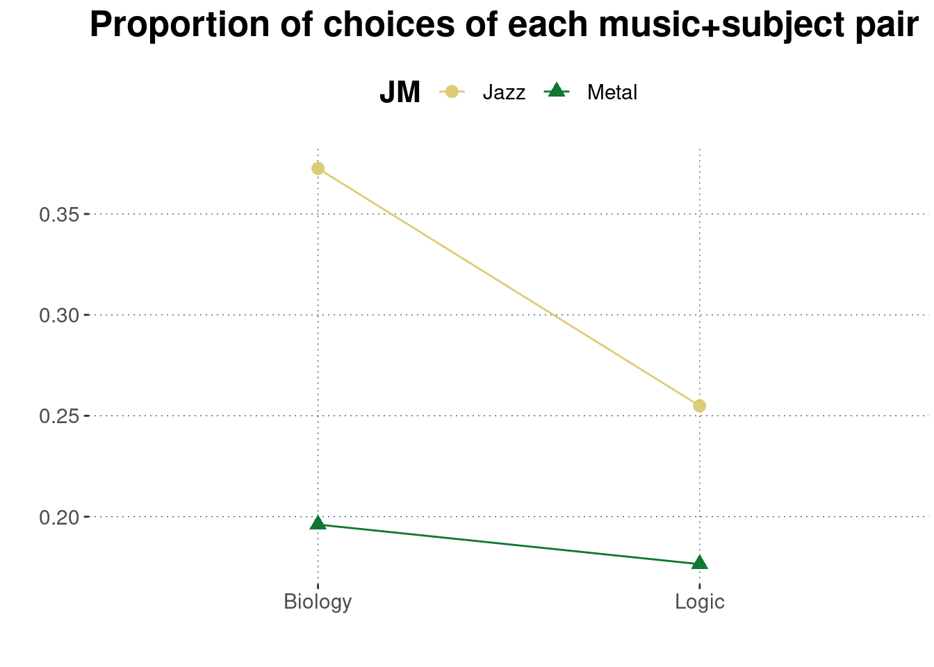
Figure 5.1: Proportions of jointly choosing a musical style and an academic subfield in the Bio-Logic Jazz-Metal data set.
Useful base R functions for obtaining counts are
tableandprop.table.↩︎