9.1 Bayes rule for parameter estimation

9.1.1 Definitions and terminology

Fix a Bayesian model \(M\) with likelihood \(P(D \mid \theta)\) for observed data \(D\) and prior over parameters \(P(\theta)\). We then update our prior beliefs \(P(\theta)\) to obtain posterior beliefs by Bayes rule:⁴⁸

\[P(\theta \mid D) = \frac{P(D \mid \theta) \ P(\theta)}{P(D)}\]

The ingredients of this equation are:

• the posterior distribution \(P(\theta \mid D)\) - our posterior beliefs about how likely each value of \(\theta\) is given \(D\);
• the likelihood function \(P(D \mid \theta)\) - how likely each observation of \(D\) is for a fixed \(\theta\);
• the prior distribution \(P(\theta)\) - our initial (prior) beliefs about how likely each value of \(\theta\) might be;
• the marginal likelihood \(P(D) = \int P(D \mid \theta) \ P(\theta) \ \text{d}\theta\) - how likely an observation of \(D\) is under our prior beliefs about \(\theta\) (a.k.a., the prior predictive probability of \(D\) according to \(M\))

A frequently used shorthand notation for probabilities is this:

\[\underbrace{P(\theta \, | \, D)}_{posterior} \propto \underbrace{P(\theta)}_{prior} \ \underbrace{P(D \, | \, \theta)}_{likelihood}\]

where the “proportional to” sign \(\propto\) indicates that the probabilities on the LHS are defined in terms of the quantity on the RHS after normalization. So, if \(F \colon X \rightarrow \mathbb{R}^+\) is a positive function of non-normalized probabilities (assuming, for simplicity, finite \(X\)), \(P(x) \propto F(x)\) is equivalent to \(P(x) = \frac{F(x)}{\sum_{x' \in X} F(x')}\).

9.1.2 The effects of prior and likelihood on the posterior

The shorthand notation for the posterior \(P(\theta \, | \, D) \propto P(\theta) \ P(D \, | \, \theta)\) makes it particularly clear that the posterior distribution is a “mix” of prior and likelihood. Let’s first explore this “mixing property” of the posterior before worrying about how to compute posteriors concretely.

We consider the case of flipping a coin with unknown bias \(\theta\) a total of \(N\) times and observing \(k\) heads (= successes). This is modeled with the Binomial Model (see Section 8.1), using priors expressed with a Beta distribution, giving us a model specification as:

\[ \begin{aligned} k & \sim \text{Binomial}(N, \theta) \\ \theta & \sim \text{Beta}(a, b) \end{aligned} \]

To study the impact of the likelihood function, we compare two data sets. The first one is the contrived “24/7” example where \(N = 24\) and \(k = 7\). The second example uses a much larger naturalistic data set stemming from the King of France example, namely \(k = 109\) for \(N = 311\). These numbers are the number of “true” responses and the total number of responses for all conditions except Condition 1, which did not involve a presupposition.

data_KoF_cleaned <- aida::data_KoF_cleaned

data_KoF_cleaned %>% 
  filter(condition != "Condition 1") %>% 
  group_by(response) %>% 
  dplyr::count()

## # A tibble: 2 × 2
## # Groups:   response [2]
##   response     n
##   <lgl>    <int>
## 1 FALSE      202
## 2 TRUE       109

The likelihood function for both data sets is plotted in Figure 9.1. The most important thing to notice is that the more data we have (as in the KoF example), the narrower the range of parameter values that make the data likely. Intuitively, this means that the more data we have, the more severely constrained the range of a posteriori plausible parameter values will be, all else equal.

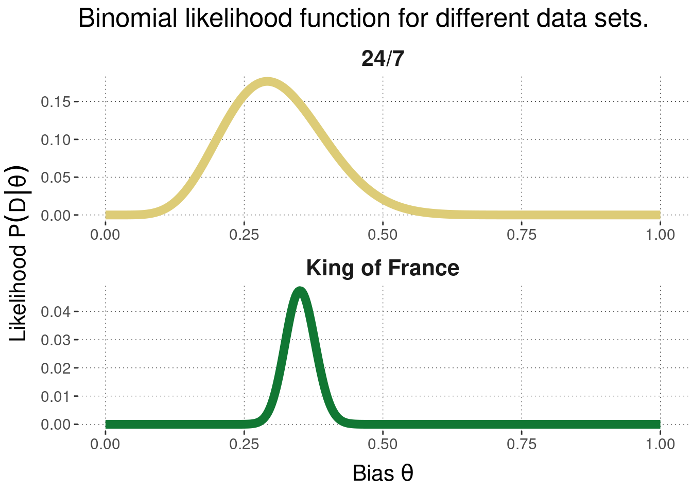
Figure 9.1: Likelihood for two examples of binomial data. The first example has \(k = 7\) and \(N = 24\). The second has \(k = 109\) and \(N = 311\).

Picking up the example from Section 8.3.2, we will consider the four types of priors show below in Figure 9.2.

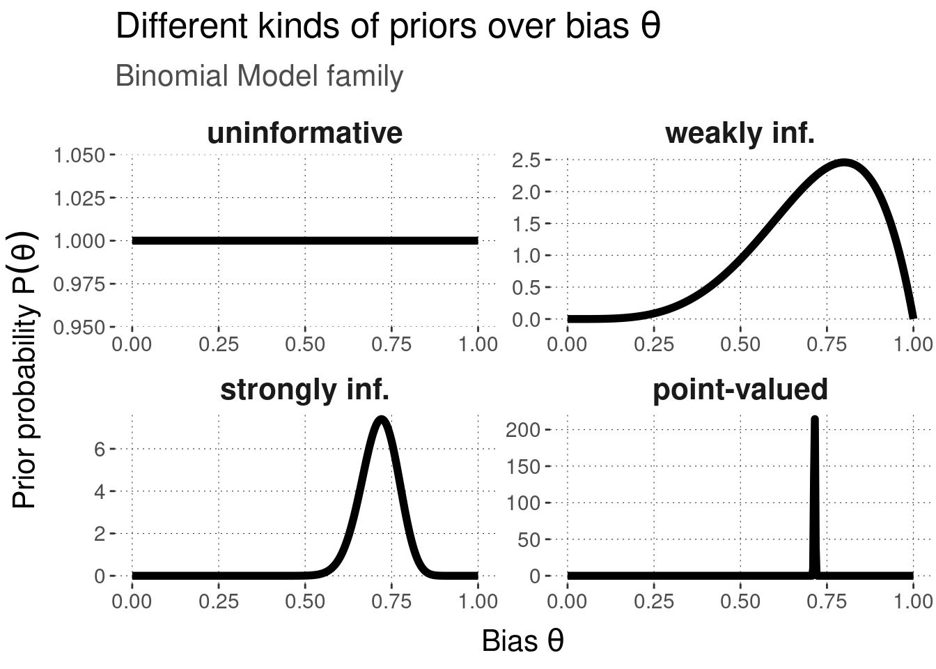
Figure 9.2: Examples of different kinds of Bayesian priors for the Binomial Model.

Combining the four different priors and the two different data sets, we see that the posterior is indeed a mix of prior and likelihood. In particular, we see that the weakly informative prior has only little effect if there are many data points (the KoF data), but does affect the posterior of the 24/7 case (compared against the uninformative prior).

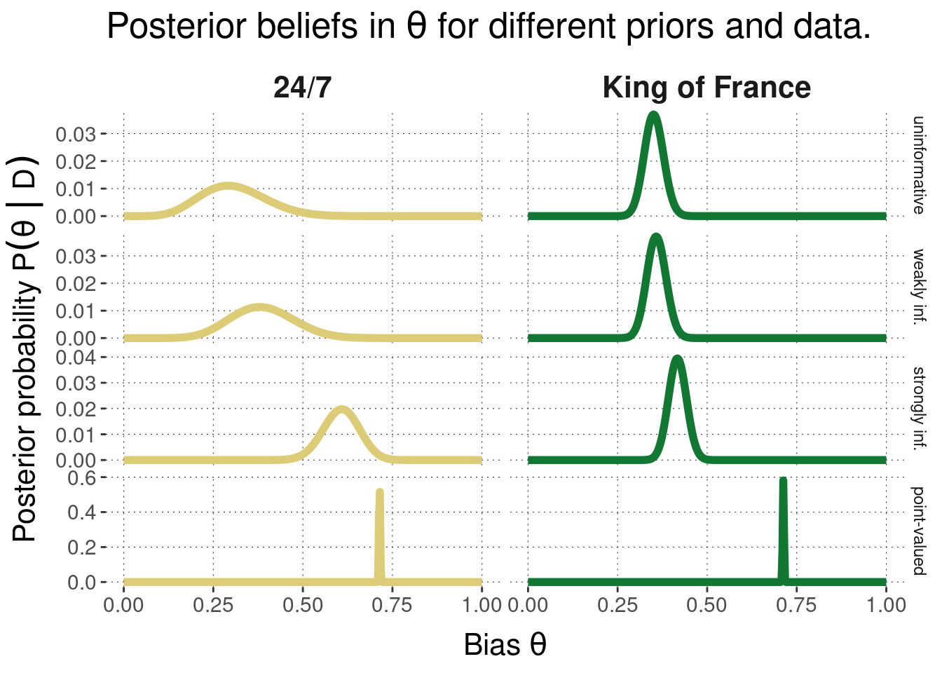
Figure 9.3: Posterior beliefs over bias parameter \(\theta\) under different priors and different data sets. We see that strongly informative priors have more influence on the posterior than weakly informative priors, and that the influence of the prior is stronger for less data than for more.

Exercise 9.1

1. Use the WebPPL code below to explore the effects of priors and different observations in the Binomial Model in order to be able to answer the questions in the second part below. Ask yourself how you need to change parameters in such a way as to:

• make the contribution of the likelihood function stronger
• make the prior more informative

// select your parameters here
var k = 7    // observed successes (heads)
var N = 24   // total flips of a coin
var a = 1    // first shape parameter of beta prior
var b = 1    // second shape parameter of beta prior
var n_samples = 50000  // number of samples for approximation
///fold:
display("Prior distribution")
var prior = function() {
  beta(a, b)
}
viz(Infer({method: "rejection", samples: n_samples}, prior))

display("\nPosterior distribution")
var posterior = function() {
  beta(k + a, N - k + b)
}
viz(Infer({method: "rejection", samples: n_samples}, posterior))
///

To make the influence of the likelihood function stronger, we need more data. Try increasing variables N and k without changing their ratio.

To make the prior more strongly informative, you should increase the shape parameters a and b.

2. Based on your explorations of the WebPPL code, which of the following statements do you think is true?

1. The prior always influences the posterior more than the likelihood.

2. The less informative the prior, the more the posterior is influenced by it.

3. The posterior is more influenced by the likelihood the less informative the prior is.

4. The likelihood always influences the posterior more than the prior.

5. The likelihood has no influence on the posterior in case of a point-valued prior (assuming a single-parameter model).

1. False

2. False

3. True

4. False

5. True

9.1.3 Computing Bayesian posteriors with conjugate priors

Bayesian posterior distributions can be hard to compute. Almost always, the prior \(P(\theta)\) is easy to compute (otherwise, we might choose a different one for practicality). Usually, the likelihood function \(P(D \mid \theta)\) is also fast to compute. Everything seems innocuous when we just write:

\[\underbrace{P(\theta \, | \, D)}_{posterior} \propto \underbrace{P(\theta)}_{prior} \ \underbrace{P(D \, | \, \theta)}_{likelihood}\]

But the real pain is the normalizing constant, i.e., the marginalized likelihood a.k.a. the “integral of doom”, which to compute can be intractable, especially if the parameter space is large and not well-behaved:

\[P(D) = \int P(D \mid \theta) \ P(\theta) \ \text{d}\theta\]

Section 9.3 will, therefore, enlarge on methods to compute or approximate the posterior distribution efficiently.

Fortunately, the computation of Bayesian posterior distributions can be quite simple in special cases. If the prior and the likelihood function cooperate, so to speak, the computation of the posterior can be as simple as sleep. The nature of the data often prescribes which likelihood function is plausible. But we have more wiggle room in the choice of the priors. If prior \(P(\theta)\) and posterior \(P(\theta \, | \, D)\) are of the same family, i.e., if they are the same kind of distribution albeit possibly with different parameterizations, we say that they conjugate. In that case, the prior \(P(\theta)\) is called conjugate prior for the likelihood function \(P(D \, | \, \theta)\) from which the posterior \(P(\theta \, | \, D)\) is derived.

Theorem 9.1 The Beta distribution is the conjugate prior of binomial likelihood. For \(\theta \sim \text{Beta}(a,b)\) as prior and data \(k\) and \(N\), the posterior is \(\theta \sim \text{Beta}(a+k, b+ N-k)\).

Proof. By construction, the posterior is: \[P(\theta \mid \langle{k, N \rangle}) \propto \text{Binomial}(k ; N, \theta) \ \text{Beta}(\theta \, | \, a, b) \]

We extend the RHS by definitions, while omitting the normalizing constants:

\[ \begin{aligned} \text{Binomial}(k ; N, \theta) \ \text{Beta}(\theta \, | \, a, b) & \propto \theta^{k} \, (1-\theta)^{N-k} \, \theta^{a-1} \, (1-\theta)^{b-1} \\ & = \theta^{k + a - 1} \, (1-\theta)^{N-k +b -1} \end{aligned} \]

This latter expression is the non-normalized Beta-distribution for parameters \(a + k\) and \(b + N - k\), so that we conclude with what was to be shown:

\[ \begin{aligned} P(\theta \mid \langle k, N \rangle) & = \text{Beta}(\theta \, | \, a + k, b+ N-k) \end{aligned} \]

 

Exercise 9.2

1. Fill in the blanks in the code below to get a plot of the posterior distribution for the coin flip scenario with \(k=20\), \(N=24\), making use of conjugacy and starting with a uniform Beta prior.

theta = seq(0, 1, length.out = 401)

as_tibble(theta) %>%
  mutate(posterior =  ____ ) %>%
  ggplot(aes(___, posterior)) +
   geom_line()

theta <- seq(0, 1, length.out = 401)

as_tibble(theta) %>%
  mutate(posterior = dbeta(theta, 21, 5)) %>%
  ggplot(aes(theta, posterior)) +
   geom_line()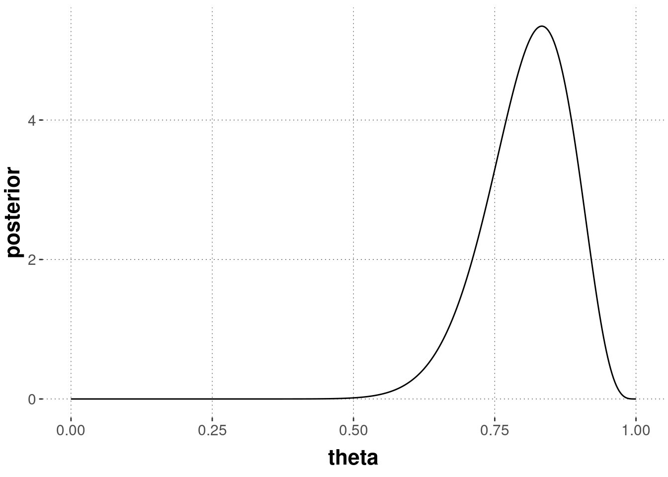

2. Suppose that Jones flipped a coin with unknown bias 30 times. She observed 20 heads. She updates her beliefs rationally with Bayes rule. Her posterior beliefs have the form of a beta distribution with parameters \(\alpha = 25\), \(\beta = 15\). What distribution and what parameter values of that distribution capture Jones’ prior beliefs before updating her beliefs with this data?

\(\text{Beta}(5,5)\)

9.1.4 Excursion: Sequential updating

Ancient wisdom has coined the widely popular proverb: “Today’s posterior is tomorrow’s prior.” Suppose we collected data from an experiment, like \(k = 7\) in \(N = 24\). Using uninformative priors at the outset, our posterior belief after the experiment is \(\theta \sim \text{Beta}(8,18)\). But now consider what happened at half-time. After half the experiment, we had \(k = 2\) and \(N = 12\), so our beliefs followed \(\theta \sim \text{Beta}(3, 11)\) at this moment in time. But using these beliefs as priors, and observing the rest of the data would consequently result in updating the prior \(\theta \sim \text{Beta}(3, 11)\) with another set of observations \(k = 5\) and \(N = 12\), giving us the same posterior belief as what we would have gotten if we updated in one swoop. Figure 9.4 shows the steps through the belief space, starting uninformed and observing one piece of data at a time (going right for each outcome of heads, down for each outcome of tails).

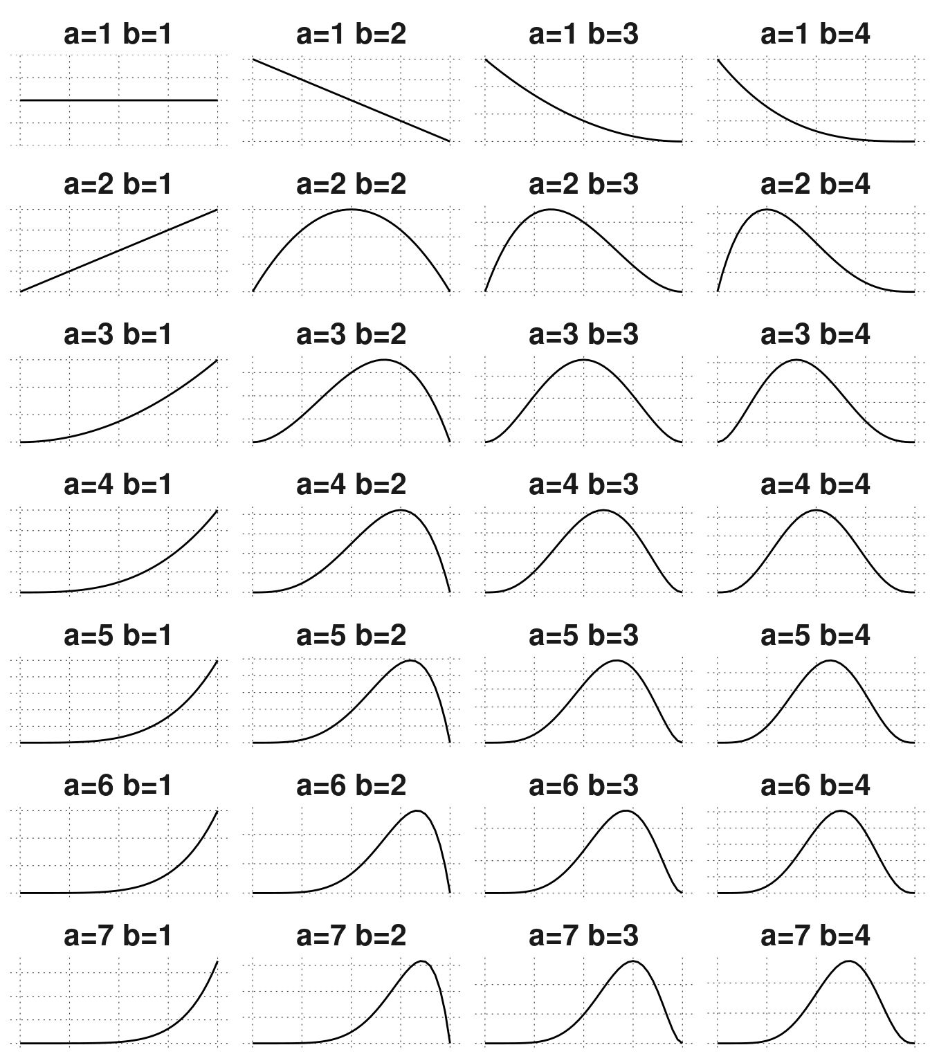
Figure 9.4: Beta distributions for different parameters. Starting from an uninformative prior (top left), we arrive at the posterior distribution in the bottom left, in any sequence of sequentially updating with the data.

This sequential updating is not a peculiarity of the Beta-Binomial case or of conjugacy. It holds in general for Bayesian inference. Sequential updating is a very intuitive property, but it is not shared by all other forms of inference from data. That Bayesian inference is sequential and commutative follows from the commutativity of multiplication of likelihoods (and the definition of Bayes rule).

Theorem 9.2 Bayesian posterior inference is sequential and commutative in the sense that for a data set \(D\) which is comprised of two mutually exclusive subsets \(D_1\) and \(D_2\) such that \(D_1 \cup D_2 = D\), we have:

\[ P(\theta \mid D ) \propto P(\theta \mid D_1) \ P(D_2 \mid \theta) \]

Proof. \[ \begin{aligned} P(\theta \mid D) & = \frac{P(\theta) \ P(D \mid \theta)}{ \int P(\theta') \ P(D \mid \theta') \text{d}\theta'} \\ & = \frac{P(\theta) \ P(D_1 \mid \theta) \ P(D_2 \mid \theta)}{ \int P(\theta') \ P(D_1 \mid \theta') \ P(D_2 \mid \theta') \text{d}\theta'} & \text{[from multiplicativity of likelihood]} \\ & = \frac{P(\theta) \ P(D_1 \mid \theta) \ P(D_2 \mid \theta)}{ \frac{k}{k} \int P(\theta') \ P(D_1 \mid \theta') \ P(D_2 \mid \theta') \text{d}\theta'} & \text{[for random positive k]} \\ & = \frac{\frac{P(\theta) \ P(D_1 \mid \theta)}{k} \ P(D_2 \mid \theta)}{\int \frac{P(\theta') \ P(D_1 \mid \theta')}{k} \ P(D_2 \mid \theta') \text{d}\theta'} & \text{[rules of integration; basic calculus]} \\ & = \frac{P(\theta \mid D_1) \ P(D_2 \mid \theta)}{\int P(\theta' \mid D_1) \ P(D_2 \mid \theta') \text{d}\theta'} & \text{[Bayes rule with } k = \int P(\theta) P(D_1 \mid \theta) \text{d}\theta ]\\ \end{aligned} \]

 

9.1.5 Posterior predictive distribution

We already learned about the prior predictive distribution of a model in Chapter 8.3.3. Remember that the prior predictive distribution of a model \(M\) captures how likely hypothetical data observations are from an a priori point of view. It was defined like this:

\[ \begin{aligned} P_M(D_{\text{pred}}) & = \sum_{\theta} P_M(D_{\text{pred}} \mid \theta) \ P_M(\theta) && \text{[discrete parameter space]} \\ P_M(D_{\text{pred}}) & = \int P_M(D_{\text{pred}} \mid \theta) \ P_M(\theta) \ \text{d}\theta && \text{[continuous parameter space]} \end{aligned} \]

After updating beliefs about parameter values in the light of observed data \(D_{\text{obs}}\), we can similarly define the posterior predictive distribution, which is analogous to the prior predictive distribution, except that it relies on the posterior over parameter values \(P_{M(\theta \mid D_{\text{obs}})}\) instead of the prior \(P_M(\theta)\):

\[ \begin{aligned} P_M(D_{\text{pred}} \mid D_{\text{obs}}) & = \sum_{\theta} P_M(D_{\text{pred}} \mid \theta) \ P_M(\theta \mid D_{\text{obs}}) && \text{[discrete parameter space]} \\ P_M(D_{\text{pred}} \mid D_{\text{obs}}) & = \int P_M(D_{\text{pred}} \mid \theta) \ P_M(\theta \mid D_{\text{obs}}) \ \text{d}\theta && \text{[continuous parameter space]} \end{aligned} \]

---

48. Since parameter estimation is only about one model, it is harmless to omit the index \(M\) in the probability notation.↩︎