16.3 [Excursion] Central Limit Theorem
The previous sections expanded on the notion of a \(p\)-value and showed how to calculate \(p\)-values for different kinds of research questions for data from repeated Bernoulli trials (= coin flips). We saw that a natural test statistic is the Binomial distribution. The Binomial distribution described the sampling distribution precisely, i.e., the sampling distribution for the frequentist Binomial Model as we set it up is the Binomial distribution. Unfortunately, there are models and types of data for which the sampling distribution is not known precisely. In these cases, frequentist statistics work with approximations to the true sampling distribution. These approximations get better the more data was observed, i.e., these are limit-approximations that hold in the limit when the amount of data observed goes towards infinity. For small samples, the error might be substantial. Rules of thumb have become conventional guides for judging when (not) to use a given approximation. Which (approximation for a) sampling distribution to use needs to be decided on a case-by-case basis.
To establish that a particular distribution is a good approximation of the true sampling distribution, the most important formal result is the Central Limit Theorem (CLT). In rough terms, the CLT says that, under certain conditions, we can use a normal distribution as an approximation of the sampling distribution.
To appreciate the CLT, let’s start with another seminal result, the Law of Large Numbers, which we had already relied on when we discussed a sample-based approach to representing probability distributions. For example, the Law of Large Numbers justifies why taking (large) samples from a random variable sufficiently approximate a mean (the most prominent Bayesian point-estimator of, e.g., a posterior approximated by samples from MCMC algorithms).
Theorem 16.2 (Law of Large Numbers) Let \(X_1, \dots, X_n\) be a sequence of \(n\) differentiable random variables with equal mean, such that \(\mathbb{E}_{X_i} = \mu_X\) for all \(1 \le i \le n\).80 As the number of samples \(n\) goes to infinity, the mean of any tuple of samples, one from each \(X_i\), convergences almost surely to \(\mu_X\):
\[ P \left(\lim_{n \rightarrow \infty} \frac{1}{n} \sum_{i = 1}^n X_i = \mu_X \right) = 1 \]
Computer simulations make the point and usefulness of this fact easier to appreciate:
# sample from a standard normal distribution (mean = 0, sd = 1)
samples <- rnorm(100000)
# collect the mean after each 10 samples & plot
tibble(
  n = seq(100, length(samples), by = 10)
  ) %>%
  group_by(n) %>%
  mutate(
  mu = mean(samples[1:n])
  ) %>%
  ggplot(aes(x = n, y = mu)) +
  geom_line()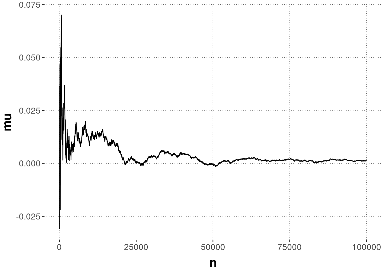
For practical purposes, think of the Central Limit Theorem as an extension of the Law of Large Numbers. While the latter tells us that, as \(n \rightarrow \infty\), the mean of repeated samples from a random variable \(X\) converges to the mean of \(X\), the Central Limit Theorem tells us something about the distribution of our estimate of \(X\)’s mean. The Central Limit Theorem tells us that the sampling distribution of the mean approximates a normal distribution for a large enough sample size.
Theorem 16.3 (Central Limit Theorem) Let \(X_1, \dots, X_n\) be a sequence of \(n\) differentiable random variables with equal mean \(\mathbb{E}_{X_i} = \mu_X\) and equal finite variance \(\text{Var}(X_i) = \sigma_X^2\) for all \(1 \le i \le n\).81 The random variable \(S_n\) which captures the distribution of the sample mean for any \(n\) is: \[ S_n = \frac{1}{n} \sum_{i=1}^n X_i \] As the number of samples \(n\) goes to infinity, the random variable \(\sqrt{n} (S_n - \mu_X)\) converges in distribution to a normal distribution with mean 0 and standard deviation \(\sigma_X\).
A proof of the CLT is not trivial, and we will omit it here. We will only point to the CLT when justifying approximations of sampling distributions, e.g., for the case of Pearson’s \(\chi^2\)-test.
Below you can explore the effect of different sample sizes and numbers of samples on the sampling distribution of the mean. Play around with the values and note how with increasing sample size and number of samples…
- …the sample mean approximates the population mean (Law of Large Numbers).
- …the distribution of sample means approximates a normal distribution (Central Limit Theorem).
To be able to simulate the CLT, we first need a population to sample from. In the drop-down menu below, you can choose how the population should be distributed, where the parameter values are fixed (e.g., if you choose “normally distributed”, the population will be distributed according to \(N(\mu = 4, \sigma = 1)\)).82 Also try out the custom option to appreciate that both concepts hold for every distribution.
In variable sample_size, you can specify how many samples you want to take from the population. number_of_samples denotes how many samples of size sample_size are taken. E.g., if number_of_samples = 5 and sample_size = 3, we would repeat the process of taking three samples from the population a total of five times. The output will show the population and sampling distribution with their means.
Though the result is more general, it is convenient to think of a natural application as the case where all \(X_i\) are samples from the exact same distribution.↩︎
As with the Law of Large Numbers, the most common application is the case where all \(X_i\) are samples from the exact same distribution.↩︎
If you want to change the default parameter values, simply click on the yellowish box and change the respective variable value. If you would like to see how different parameter values generally affect a given distribution, you should take a look at Appendix B.↩︎