15.2 Logistic regression

Suppose \(y \in \{0,1\}^n\) is an \(n\)-placed vector of binary outcomes, and \(X\) a predictor matrix for a linear regression model. A Bayesian logistic regression model has the following form:

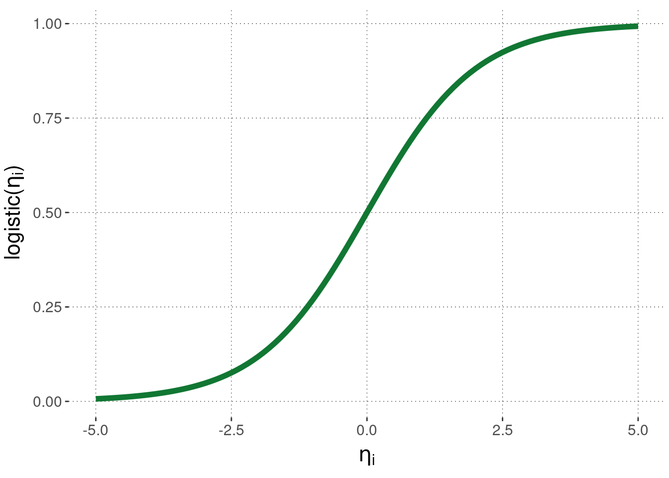
\[ \begin{align*} \beta, \sigma & \sim \text{some prior} \\ \xi & = X \beta && \text{[linear predictor]} \\ \eta_i & = \text{logistic}(\xi_i) && \text{[predictor of central tendency]} \\ y_i & \sim \text{Bernoulli}(\eta_i) && \text{[likelihood]} \\ \end{align*} \] The logistic function used as a link function is a function in \(\mathbb{R} \rightarrow [0;1]\), i.e., from the reals to the unit interval. It is defined as:

\[\text{logistic}(\xi_i) = (1 + \exp(-\xi_i))^{-1}\] It’s shape (a sigmoid, or S-shaped curve) is this:

We use the Simon task data as an example application. So far we only tested the first of two hypotheses about the Simon task data, namely the hypothesis relating to reaction times. The second hypothesis which arose in the context of the Simon task refers to the accuracy of answers, i.e., the proportion of “correct” choices:

\[ \text{Accuracy}_{\text{correct},\ \text{congruent}} > \text{Accuracy}_{\text{correct},\ \text{incongruent}} \] Notice that correctness is a binary categorical variable. Therefore, we use logistic regression to test this hypothesis.

Here is how to set up a logistic regression model with brms. The only thing that is new here is that we specify explicitly the likelihood function and the (inverse!) link function.⁷⁰ This is done using the syntax family = bernoulli(link = "logit"). For later hypothesis testing we also use proper priors and take samples from the prior as well.

fit_brms_ST_Acc = brm(
  # regress 'correctness' against 'condition'
  formula = correctness ~ condition, 
  # specify link and likeihood function
  family = bernoulli(link = "logit"),
  # which data to use
  data = aida::data_ST %>% 
    # 'reorder' answer categories (making 'correct' the target to be explained)
    mutate(correctness = correctness == 'correct'),
  # weakly informative priors (slightly conservative)
  #   for `class = 'b'` (i.e., all slopes)
  prior = prior(student_t(1, 0, 2),  class = 'b'),
  # also collect samples from the prior (for point-valued testing)
  sample_prior = 'yes',
  # take more than the usual samples (for numerical stability of testing)
  iter = 20000
)

The Bayesian summary statistics of the posterior samples of values for regression coefficients are:

summary(fit_brms_ST_Acc)$fixed[,c("l-95% CI", "Estimate", "u-95% CI")]

##                        l-95% CI   Estimate   u-95% CI
## Intercept             3.1067020  3.2042928  3.3059530
## conditionincongruent -0.8496013 -0.7260651 -0.6050912

What do these specific numerical estimates for coefficients mean? The mean estimate for the linear predictor \(\xi_\text{cong}\) for the “congruent” condition is roughly 3.204. The mean estimate for the linear predictor \(\xi_\text{inc}\) for the “incongruent” condition is roughly 3.204 + -0.726, so roughly 2.478. The central predictors corresponding to these linear predictors are:

\[ \begin{align*} \eta_\text{cong} & = \text{logistic}(3.204) \approx 0.961 \\ \eta_\text{incon} & = \text{logistic}(2.478) \approx 0.923 \end{align*} \]

These central estimates for the latent proportion of “correct” answers in each condition tightly match the empirically observed proportion of “correct” answers in the data:

proportions_correct_ST <- aida::data_ST %>% 
  group_by(condition, correctness) %>% 
  dplyr::count() %>% 
  group_by(condition) %>% 
  mutate(proportion_correct = (n / sum(n)) %>% round(3)) %>% 
  filter( correctness == "correct") %>% 
  select(-n, -correctness) 
proportions_correct_ST

## # A tibble: 2 × 2
## # Groups:   condition [2]
##   condition   proportion_correct
##   <chr>                    <dbl>
## 1 congruent                0.961
## 2 incongruent              0.923

Testing hypothesis for a logistic regression model is the exact same as for a standard regression model. And so, we find very strong support for hypothesis 2, suggesting that (given model and data), there is reason to believe that the accuracy in incongruent trials is lower than in congruent trials.

brms::hypothesis(fit_brms_ST_Acc, "conditionincongruent < 0")

## Hypothesis Tests for class b:
##                 Hypothesis Estimate Est.Error CI.Lower CI.Upper Evid.Ratio
## 1 (conditionincongr... < 0    -0.73      0.06    -0.83    -0.62        Inf
##   Post.Prob Star
## 1         1    *
## ---
## 'CI': 90%-CI for one-sided and 95%-CI for two-sided hypotheses.
## '*': For one-sided hypotheses, the posterior probability exceeds 95%;
## for two-sided hypotheses, the value tested against lies outside the 95%-CI.
## Posterior probabilities of point hypotheses assume equal prior probabilities.

Notice that the logit function is the inverse of the logistic function.↩︎