B.1 Selected continuous distributions of random variables
B.1.1 Normal distribution
One of the most important distribution families is the Gaussian or normal family because it fits many natural phenomena. Furthermore, the sampling distributions of many estimators depend on the normal distribution either because they are derived from normally distributed random variables or because they can be asymptotically approximated by a normal distribution for large samples (Central limit theorem).
Distributions of the normal family are symmetric with range \((-\infty,+\infty)\) and have two parameters \(\mu\) and \(\sigma\), respectively referred to as the mean and the standard deviation of the normal random variable. These parameters are examples of location and scale parameters. The normal distribution is located at \(\mu\), and the choice of \(\sigma\) scales its width. The distribution is symmetric, with most observations lying around the central peak \(\mu\) and more extreme values being further away depending on \(\sigma\).
\[X \sim Normal(\mu,\sigma) \ \ \text{, or alternatively written as: } \ \ X \sim \mathcal{N}(\mu,\sigma) \]
Figure B.1 shows the probability density function of three normally distributed random variables with different parameters. Figure B.2 shows the corresponding cumulative function of the three normal distributions.
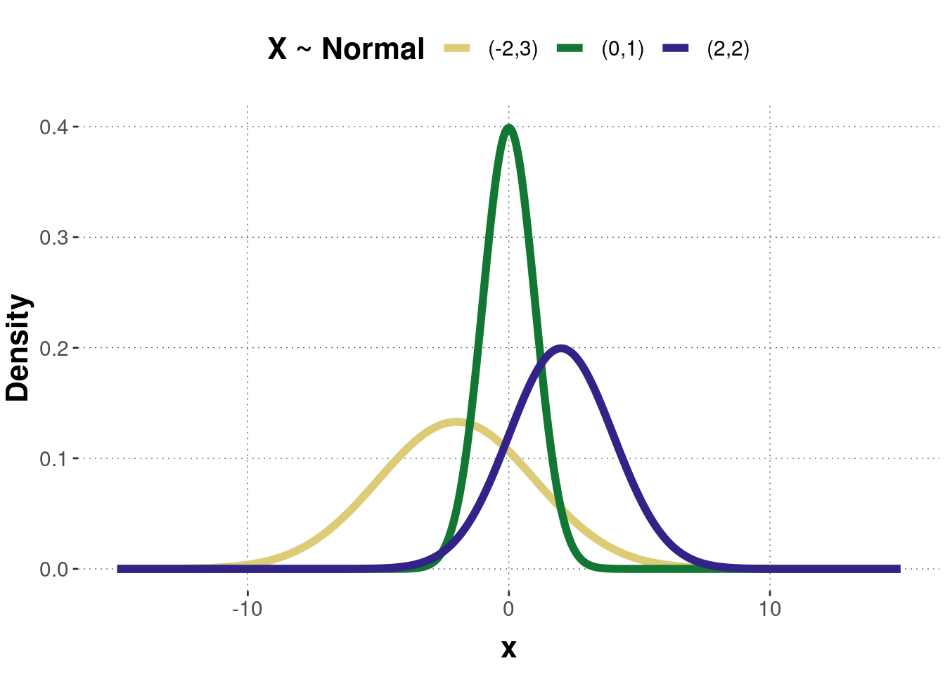
Figure B.1: Examples of a probability density function of the normal distribution. Numbers in legend represent parameter pairs \((\mu, \sigma)\).
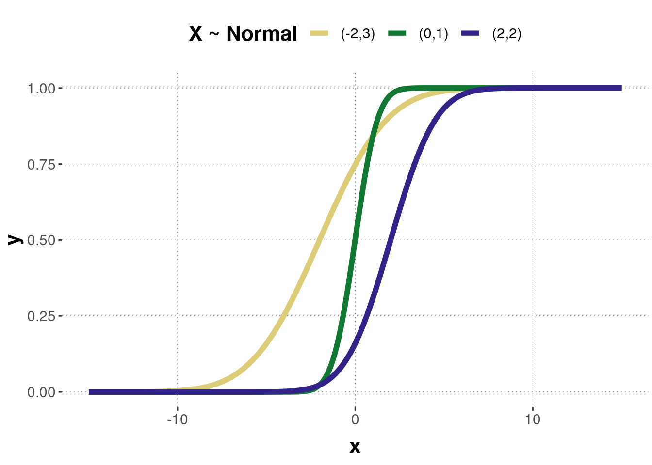
Figure B.2: The cumulative distribution functions of the normal distributions corresponding to the previous probability density functions.
Probability density function
\[f(x)=\frac{1}{\sigma\sqrt{2\pi}}\exp\left(-0.5\left(\frac{x-\mu}{\sigma}\right)^2\right)\]
Cumulative distribution function
\[F(x)=\int_{-\inf}^{x}f(t)dt\]
Expected value \(E(X)=\mu\)
Variance \(Var(X)=\sigma^2\)
Deviation and Coverage The normal distribution is often associated with the 68-95-99.7 rule. The values refer to the probability of a random data point landing within one, two or three standard deviations of the mean (Figure B.3 depicts these three intervals). For example, about 68% of the values drawn from a normal distribution are within one standard deviation \(\sigma\) away from the mean \(\mu\).
- \(P(\mu-\sigma \leq X \leq \mu+\sigma) = 0.6827\)
- \(P(\mu-2\sigma \leq X \leq \mu+2\sigma) = 0.9545\)
- \(P(\mu-3\sigma \leq X \leq \mu+3\sigma) = 0.9973\)
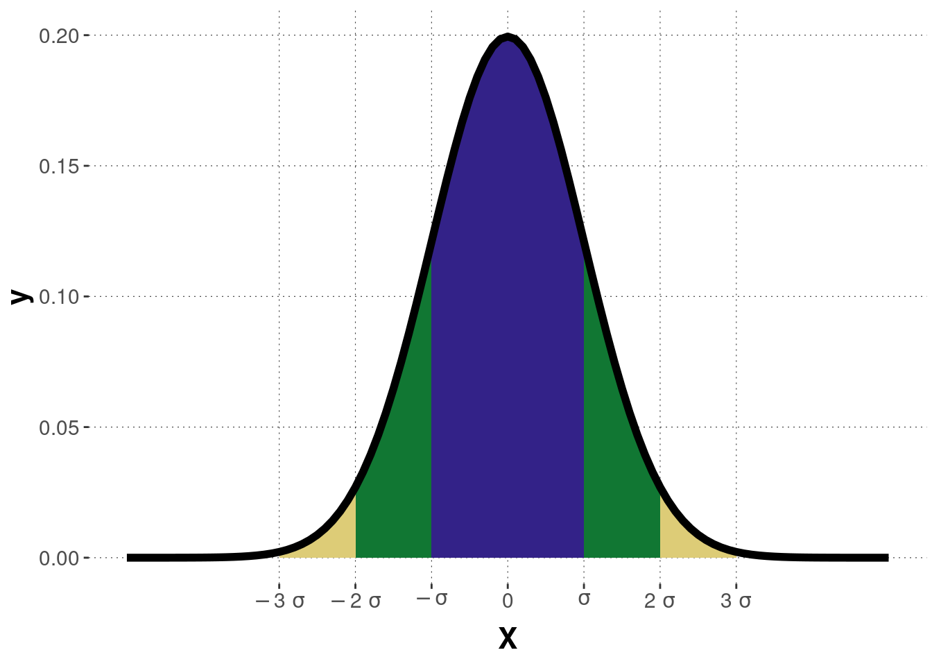
Figure B.3: The coverage of a normal distribution.
Z-transformation / standardization
A special case of normally distributed random variables is the standard normal distributed variable with \(\mu=0\) and \(\sigma=1\): \(Y\sim Normal(0,1)\). Each normal distribution \(X\) can be converted into a standard normal distribution \(Z\) by z-transformation (see equation below):
\[Z=\frac{X-\mu}{\sigma}\]
The advantage of standardization is that values from different scales can be compared because they become scale-independent by z-transformation.
Alternative parameterization
Often a normal distribution is parameterized in terms of its mean \(\mu\) and variance \(\sigma^2\). This is clear, from writing \(X\sim Normal(\mu, \sigma^2)\), instead of \(X\sim Normal(\mu, \sigma)\).
Linear transformations
- If normal random variable \(X\sim Normal(\mu, \sigma^2)\) is linearly transformed by \(Y=a*X+b\), then the new random variable \(Y\) is again normally distributed with \(Y \sim Normal(a\mu+b,a^2\sigma^2)\).
- Are \(X\sim Normal(\mu_x, \sigma^2)\) and \(Y\sim Normal(\mu_y, \sigma^2)\) normally distributed and independent, then their sum is again normally distributed with \(X+Y \sim Normal(\mu_x+\mu_y, \sigma_x^2+\sigma_y^2)\).
B.1.1.1 Hands-on
Here’s WebPPL code to explore the effect of different parameter values on a normal distribution:
var mu = 2;            // mean
var sigma = 3;         // standard deviation
var n_samples = 30000; // number of samples used for approximation
///fold:
viz(repeat(n_samples, function(x) {gaussian({mu: mu, sigma: sigma})}));
///
B.1.2 Chi-squared distribution
The \(\chi^2\)-distribution is widely used in hypothesis testing in inferential statistics because many test statistics are approximately distributed as \(\chi^2\)-distribution.
The \(\chi^2\)-distribution is directly related to the standard normal distribution: The sum of the squares of \(n\) independent and standard normally distributed random variables \(X_1,X_2,...,X_n\) is distributed according to a \(\chi^2\)-distribution with \(n\) degrees of freedom:
\[Y=X_1^2+X_2^2+...+X_n^2.\]
The \(\chi^2\)-distribution is a skewed probability distribution with range \([0,+\infty)\) and only one parameter \(n\), the degrees of freedom (if \(n=1\), then the range is \((0,+\infty)\)):
\[X\sim \chi^2(n).\]
Figure B.4 shows the probability density function of three \(\chi^2\)-distributed random variables with different values for the parameter. Notice that with increasing degrees of freedom, the \(\chi^2\)-distribution can be approximated by a normal distribution (for \(n \geq 30\)). Figure B.5 shows the corresponding cumulative function of the three \(\chi^2\)-density distributions.
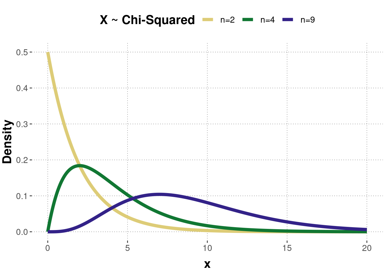
Figure B.4: Examples of a probability density function of the chi-squared distribution.
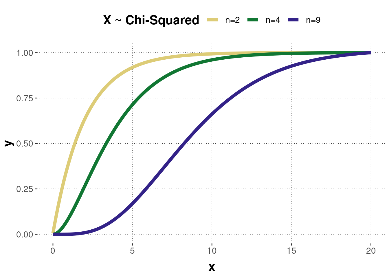
Figure B.5: The cumulative distribution functions of the chi-squared distributions corresponding to the previous probability density functions.
Probability density function \[f(x)=\begin{cases}\frac{x^{\frac{n}{2}-1}e^{-\frac{x}{2}}}{2^{\frac{n}{2}}\Gamma (\frac{n}{2})} &\textrm{ for }x>0,\\ 0 &\textrm{ otherwise.}\end{cases}\] where \(\Gamma (\frac{n}{2})\) denotes the gamma function.
Cumulative distribution function \[F(x)=\frac{\gamma (\frac{n}{2},\frac{x}{2})}{\Gamma \frac{n}{2}},\] with \(\gamma(s,t)\) being the lower incomplete gamma function: \[\gamma(s,t)=\int_0^t t^{s-1}e^{-t} dt.\]
Expected value \(E(X)=n\)
Variance \(Var(X)=2n\)
Transformations The sum of two \(\chi^2\)-distributed random variables \(X \sim \chi^2(m)\) and \(Y \sim \chi^2(n)\) is again a \(\chi^2\)-distributed random variable with \(X+Y=\chi^2(m+n)\).
B.1.2.1 Hands-on
Here’s WebPPL code to explore the effect of different parameter values on a \(\chi^2\)-distribution:
var df = 1;            // degrees of freedom
var n_samples = 30000; // number of samples used for approximation
///fold:
var chisq = function(nu) {
  var y = sample(Gaussian({mu: 0, sigma: 1}));
  if (nu == 1) {
    return y*y;
  } else {
    return y*y+chisq(nu-1);
  }
}

viz(repeat(n_samples, function(x) {chisq(df)}));
///
B.1.3 F-distribution
The F-distribution, named after R.A. Fisher, is particularly used in regression and variance analysis. It is defined by the ratio of two \(\chi^2\)-distributed random variables \(X\sim \chi^2(m)\) and \(Y\sim \chi^2(n)\), each divided by its degrees of freedom:
\[F=\frac{\frac{X}{m}}{\frac{Y}{n}}.\] The F-distribution is a continuous skewed probability distribution with range \((0,+\infty)\) and two parameters \(m\) and \(n\), corresponding to the degrees of freedom of the two \(\chi^2\)-distributed random variables:
\[X \sim F(m,n).\]
Figure B.6 shows the probability density function of three F-distributed random variables with different parameter values. For a small number of degrees of freedom, the density distribution is skewed to the left side. When the number increases, the density distribution gets more and more symmetric. Figure B.7 shows the corresponding cumulative function of the three density distributions.
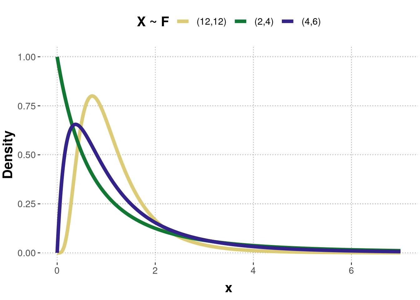
Figure B.6: Examples of a probability density function of the F-distribution. Pairs of numbers in the legend are parameters \((m,n)\).
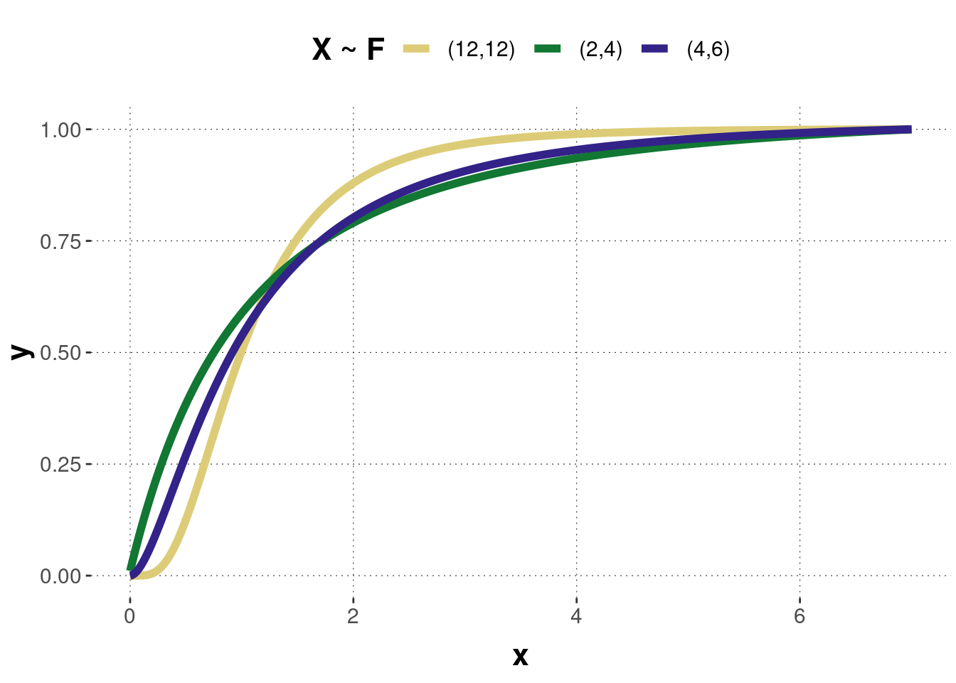
Figure B.7: The cumulative distribution functions of the F-distributions corresponding to the previous probability density functions.
Probability density function \[F(x)=m^{\frac{m}{2}}n^{\frac{n}{2}} \cdot \frac{\Gamma (\frac{m+n}{2})}{\Gamma (\frac{m}{2})\Gamma (\frac{n}{2})} \cdot \frac{x^{\frac{m}{2}-1}}{(mx+n)^{\frac{m+n}{2}}} \textrm{ for } x>0,\] where \(\Gamma(x)\) denotes the gamma function.
Cumulative distribution function \[F(x)=I\left(\frac{m \cdot x}{m \cdot x+n},\frac{m}{2},\frac{n}{2}\right),\] with \(I(z,a,b)\) being the regularized incomplete beta function: \[I(z,a,b)=\frac{1}{B(a,b)} \cdot \int_0^z t^{a-1}(1-t)^{b-1} dt.\]
Expected value \(E(X) = \frac{n}{n-2}\) (for \(n \geq 3\))
Variance \(Var(X) = \frac{2n^2(n+m-2)}{m(n-4)(n-2)^2}\) (for \(n \geq 5\))
B.1.3.1 Hands-on
Here’s WebPPL code to explore the effect of different parameter values on an F-distribution:
var df1 = 12;           // degrees of freedom 1
var df2 = 12;           // degrees of freedom 2
var n_samples = 30000;  // number of samples used for approximation
///fold:
var chisq = function(nu) {
  var y = sample(Gaussian({mu: 0, sigma: 1}));
  if (nu == 1) {
    return y*y;
  } else {
    return y*y+chisq(nu-1);
  }
}

var F = function(nu1, nu2) {
  var X = chisq(nu1)/nu1;
  var Y = chisq(nu2)/nu2;
  return X/Y;
}

viz(repeat(n_samples, function(x) {F(df1, df2)}));
///
B.1.4 Student’s t-distribution
The Student’s \(t\)-distribution, or just \(t\)-distribution for short, was discovered by William S. Gosset in 1908 (Vallverdú 2016), who published his work under the pseudonym “Student”. He worked at the Guinness factory and had to deal with the problem of small sample sizes, where using a normal distribution as an approximation can be too crude. To overcome this problem, Gosset conceived of the \(t\)-distribution. Accordingly, this distribution is used in particular when the sample size is small and the variance unknown, which is often the case in reality. Its shape resembles the normal bell shape and has a peak at zero, but the \(t\)-distribution is a bit lower and wider (bigger tails) than the normal distribution.
The standard \(t\)-distribution consists of a standard-normally distributed random variable \(X \sim \text{Normal}(0,1)\) and a \(\chi^2\)-distributed random variable \(Y \sim \chi^2(n)\) (\(X\) and \(Y\) are independent):
\[T = \frac{X}{\sqrt{Y / n}}.\] The \(t\)-distribution has the range \((-\infty,+\infty)\) and one parameter \(\nu\), the degrees of freedom. The degrees of freedom can be calculated by the sample size \(n\) minus one: \[t \sim \text{Student-}t(\nu = n -1).\]
Figure B.8 shows the probability density function of three \(t\)-distributed random variables with different parameters, and Figure B.9 shows the corresponding cumulative functions. Notice that for small degrees of freedom \(\nu\), the \(t\)-distribution has bigger tails. This is because the \(t\)-distribution was specially designed to provide more conservative test results when analyzing small samples. When the degrees of freedom increase, the \(t\)-distribution approaches a normal distribution. For \(\nu \geq 30\), this approximation is quite good.
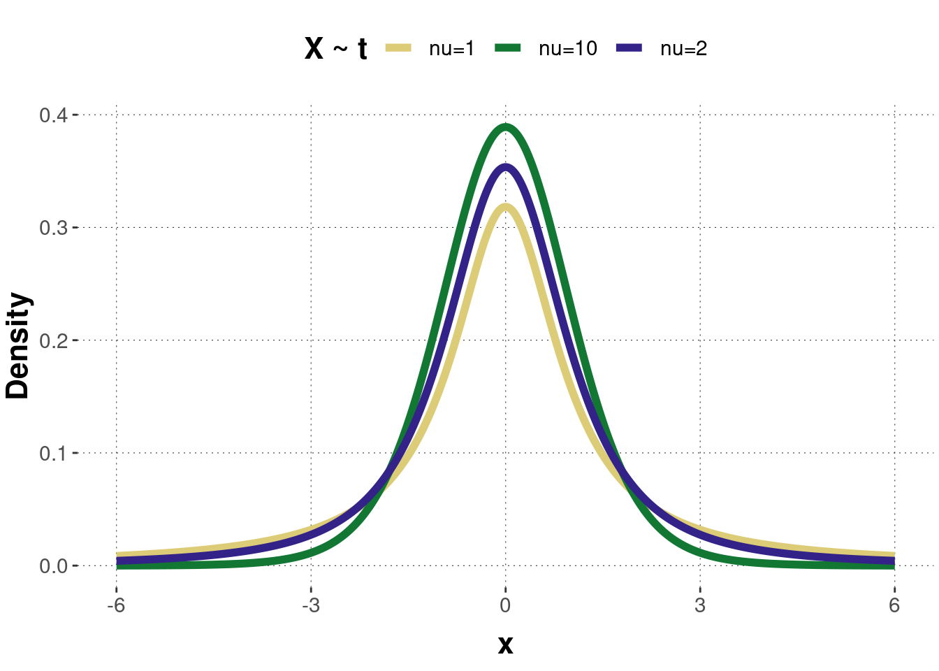
Figure B.8: Examples of a probability density function of the \(t\)-distribution.
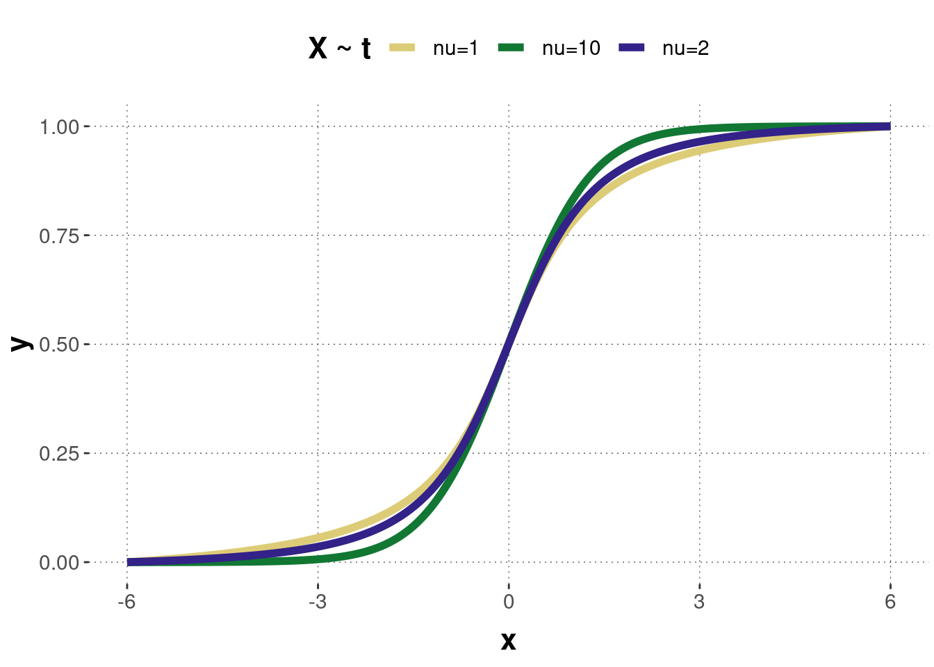
Figure B.9: The cumulative distribution functions of the \(t\)-distributions corresponding to the previous probability density functions.
Probability density function \[ f(x, \nu)=\frac{\Gamma(\frac{\nu+1}{2})}{\sqrt{\nu\pi} \cdot \Gamma(\frac{\nu}{2})}\left(1+\frac{x^2}{\nu}\right)^{-\frac{\nu+1}{2}},\] with \(\Gamma(x)\) denoting the gamma function.
Cumulative distribution function \[F(x, \nu)=I\left(\frac{x+\sqrt{x^2+\nu}}{2\sqrt{x^2+\nu}},\frac{\nu}{2},\frac{\nu}{2}\right),\] where \(I(z,a,b)\) denotes the regularized incomplete beta function: \[I(z,a,b)=\frac{1}{B(a,b)} \cdot \int_0^z t^{a-1}(1-t)^{b-1} \text{d}t.\]
Expected value \(E(X) = 0\)
Variance \(Var(X) = \frac{n}{n-2}\) (for \(n \geq 30\))
B.1.4.1 Hands-on
Here’s WebPPL code to explore the effect of different parameter values on a \(t\)-distribution:
var df = 3;            // degrees of freedom
var n_samples = 30000; // number of samples used for approximation
///fold:
var chisq = function(nu) {
  var y = sample(Gaussian({mu: 0, sigma: 1}));
  if (nu == 1) {
    return y*y;
  } else {
    return y*y+chisq(nu-1);
  }
}

var t = function(nu) {
  var X = sample(Gaussian({mu: 0, sigma: 1}));
  var Y = chisq(nu);
  return X/Math.sqrt(Y/nu);
}

viz(repeat(n_samples, function(x) {t(df)}));
///
Beyond the standard \(t\)-distribution there are also generalized \(t\)-distributions taking three parameters \(\nu\), \(\mu\) and \(\sigma\), where the latter two are just the mean and the standard deviations, similar to the case of the normal distribution.
B.1.5 Beta distribution
The beta distribution creates a continuous distribution of numbers between 0 and 1. Therefore, this distribution is useful if the uncertain quantity is bounded by 0 and 1 (or 100%), is continuous, and has a single mode. In Bayesian Data Analysis, the beta distribution has a special standing as prior distribution for a Bernoulli or binomial likelihood. The reason for this is that a combination of a beta prior and a Bernoulli (or binomial) likelihood results in a posterior distribution with the same form as the beta distribution. Such priors are referred to as conjugate priors (see Chapter 9.1.3).
A beta distribution has two parameters \(a\) and \(b\) (sometimes also represented in Greek letters \(\alpha\) and \(\beta\)):
\[X \sim Beta(a,b).\]
The two parameters can be interpreted as the number of observations made, such that: \(n=a+b\). If \(a\) and \(b\) get bigger, the beta distribution gets narrower. If only \(a\) gets bigger, the distribution moves rightward, and if only \(b\) gets bigger, the distribution moves leftward. As the parameters define the shape of the distribution, they are also called shape parameters. A Beta(1,1) is equivalent to a uniform distribution. Figure B.10 shows the probability density function of four beta distributed random variables with different parameter values. Figure B.11 shows the corresponding cumulative functions.
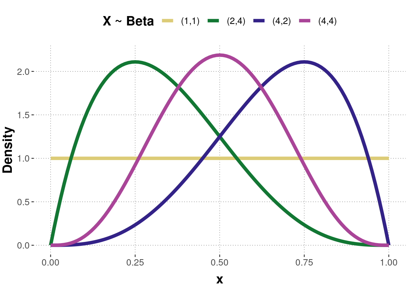
Figure B.10: Examples of a probability density function of the beta distribution. Pairs of numbers in the legend represent parameters \((a, b)\).
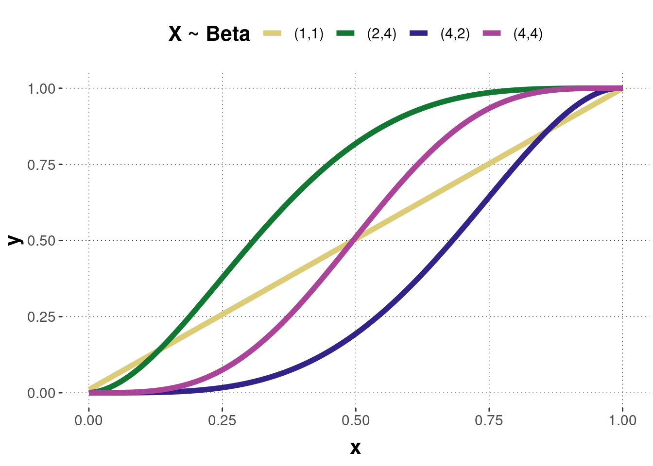
Figure B.11: The cumulative distribution functions of the beta distributions corresponding to the previous probability density functions.
Probability density function
\[f(x)=\frac{\theta^{(a-1)} (1-\theta)^{(b-1)}}{B(a,b)},\] where \(B(a,b)\) is the beta function:
\[B(a,b)=\int^1_0 \theta^{(a-1)} (1-\theta)^{(b-1)}d\theta.\]
Cumulative distribution function
\[F(x)=\frac{B(x;a,b)}{B(a,b)},\] where \(B(x;a,b)\) is the incomplete beta function:
\[B(x;a,b)=\int^x_0 t^{(a-1)} (1-t)^{(b-1)} dt,\]
and \(B(a,b)\) the (complete) beta function:
\[B(a,b)=\int^1_0 \theta^{(a-1)} (1-\theta)^{(b-1)}d\theta.\]
Expected value
Mean: \(E(X)=\frac{a}{a+b}\)
Mode: \(\omega=\frac{(a-1)}{a+b-2}\)
Variance
Variance: \(Var(X)=\frac{ab}{(a+b)^2(a+b+1)}\)
Concentration: \(\kappa=a+b\) (related to variance such that the bigger \(a\) and \(b\) are, the narrower the distribution)
Reparameterization of the beta distribution Sometimes it is helpful (and more intuitive) to write the beta distribution in terms of its mode \(\omega\) and concentration \(\kappa\) instead of \(a\) and \(b\):
\[Beta(a,b)=Beta(\omega(\kappa-2)+1, (1-\omega)(\kappa-2)+1), \textrm{ for } \kappa > 2.\]
B.1.5.1 Hands-on
Here’s WebPPL code to explore the effect of different parameter values on a beta distribution:
var a = 2;             // shape parameter alpha
var b = 4;             // shape parameter beta
var n_samples = 30000; // number of samples used for approximation
///fold:
viz(repeat(n_samples, function(x) {beta({a: a, b: b})}));
///
B.1.6 Uniform distribution
The (continuous) uniform distribution takes values within a specified range \(a\) and \(b\) that have constant probability. Due to its shape, the distribution is also sometimes called rectangular distribution. The uniform distribution is common for random number generation. In Bayesian Data Analysis, it is often used as prior distribution to express ignorance. This can be thought of in the following way: When different events are possible, but no (reliable) information exists about their probability of occurrence, the most conservative (and also intuitive) choice would be to assign probability in such a way that all events are equally likely to occur. The uniform distribution models this intuition and generates a completely random number in some interval \([a,b]\).
The distribution is specified by two parameters: the endpoints \(a\) (minimum) and \(b\) (maximum).
\[X \sim Uniform(a,b) \ \ \text{or alternativelly written as: } \ \ \mathcal{U}(a,b)\]
When \(a=0\) and \(b=1\), the distribution is referred to as standard uniform distribution. Figure B.12 shows the probability density function of two uniformly distributed random variables with different parameter values. Figure B.13 shows the corresponding cumulative functions.
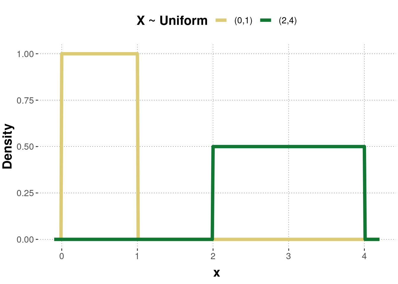
Figure B.12: Examples of a probability density function of the uniform distribution. Pairs of numbers in the legend are parameter values \((a,b)\).
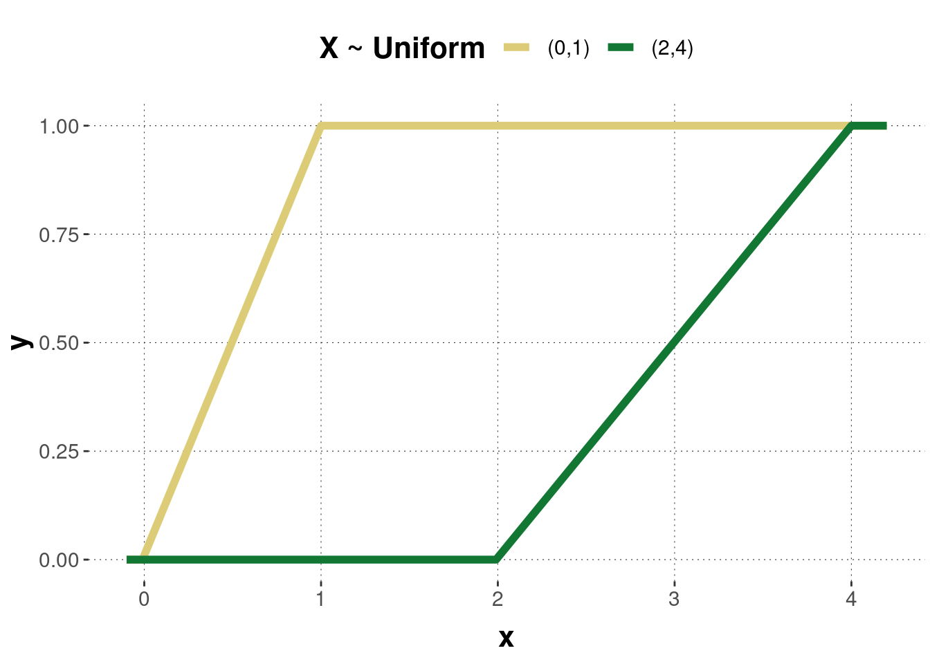
Figure B.13: The cumulative distribution functions of the uniform distributions corresponding to the previous probability density functions.
Probability density function
\[f(x)=\begin{cases} \frac{1}{b-a} &\textrm{ for } x \in [a,b],\\0 &\textrm{ otherwise.}\end{cases}\]
Cumulative distribution function
\[F(x)=\begin{cases}0 & \textrm{ for } x<a,\\\frac{x-a}{b-a} &\textrm{ for } a\leq x < b,\\ 1 &\textrm{ for }x \geq b. \end{cases}\]
Expected value \(E(X)=\frac{a+b}{2}\)
Variance \(Var(X)=\frac{(b-a)^2}{12}\)
B.1.6.1 Hands-on
Here’s WebPPL code to explore the effect of different parameter values on a uniform distribution:
var a = 0;             // lower bound
var b = 1;             // upper bound (> a)
var n_samples = 30000; // number of samples used for approximation
///fold:
viz(repeat(n_samples, function(x) {uniform({a: a, b: b})}));
///
B.1.7 Dirichlet distribution
The Dirichlet distribution is a multivariate generalization of the beta distribution: While the beta distribution is a distribution over binomials, the Dirichlet is a distribution over multinomials.
It can be used in any situation where an entity has to necessarily fall into one of \(n+1\) mutually exclusive subclasses, and the goal is to study the proportion of entities belonging to the different subclasses.
The Dirichlet distribution is commonly used as prior distribution in Bayesian statistics, as this family is a conjugate prior for the categorical distribution and the multinomial distribution.
The Dirichlet distribution \(\mathcal{Dir}(\alpha)\) is a family of continuous multivariate probability distributions, parameterized by a vector \(\alpha\) of positive reals. Thus, it is a distribution with \(k\) positive parameters \(\alpha^k\) with respect to a \(k\)-dimensional space.
\[X \sim \mathcal{Dirichlet}(\boldsymbol{\alpha})\]
The probability density function (see formula below) of the Dirichlet distribution for \(k\) random variables is a \(k-1\) dimensional probability simplex that exists on a \(k\)-dimensional space. How does the parameter \(\alpha\) influence the Dirichlet distribution?
- Values of \(\alpha_i<1\) can be thought of as anti-weight that pushes away \(x_i\) toward extremes (see upper left panel of Figure B.14).
- If \(\alpha_1=...=\alpha_k=1\), then the points are uniformly distributed (see upper right panel).
- Higher values of \(\alpha_i\) lead to greater “weight” of \(X_i\) and a greater amount of the total “mass” assigned to it (see lower left panel).
- If all \(\alpha_i\) are equal, the distribution is symmetric (see lower right panel for an asymmetric distribution).
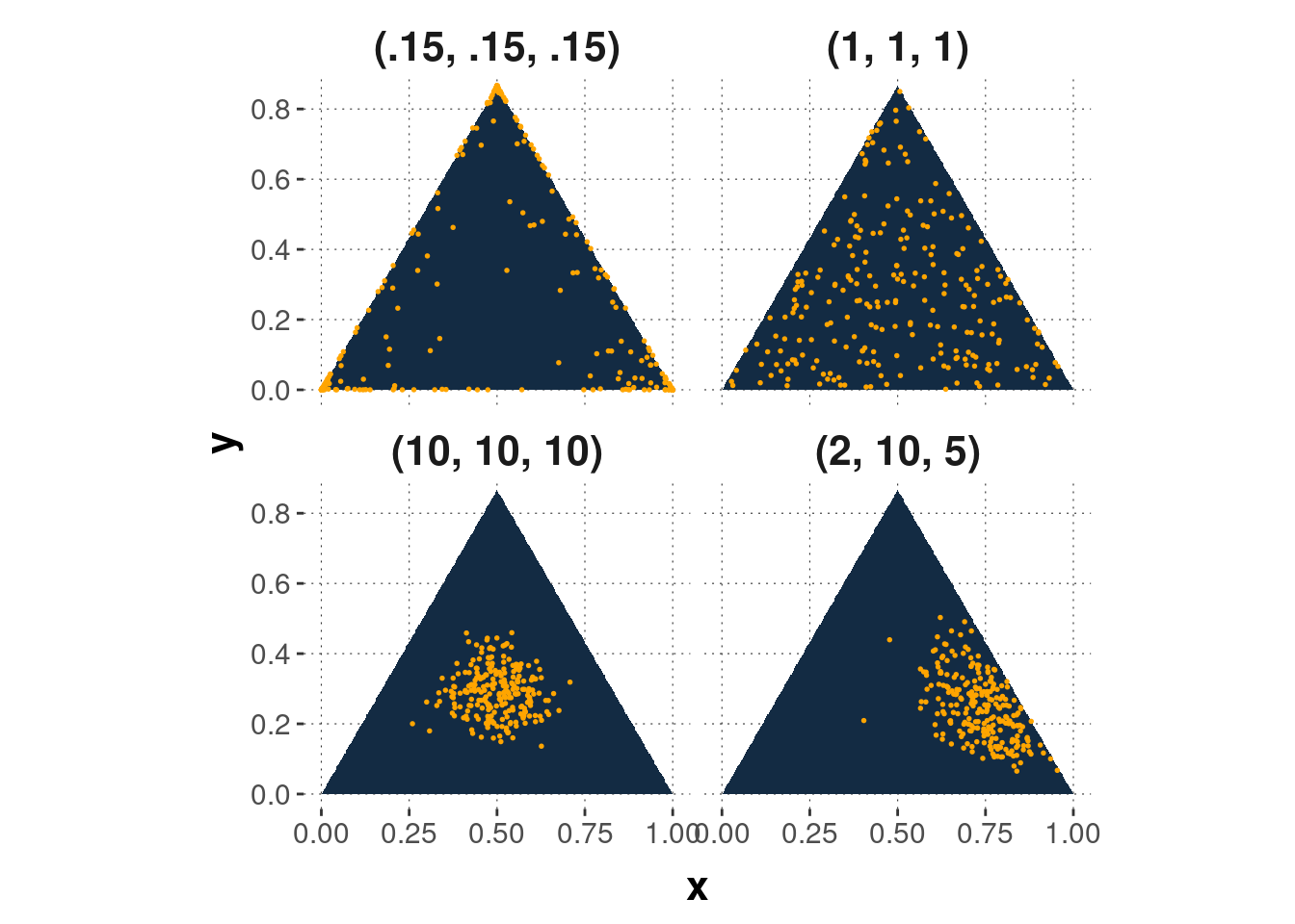
Figure B.14: Examples of a probability density function of the Dirichlet distribution with dimension \(k\) for different parameter vectors \(\alpha\).
Probability density function
\[f(x)=\frac{\Gamma\left(\sum_{i=1}^{n+1} \alpha_i\right)}{\prod_{i=1}^{n+1}\Gamma(\alpha_i)}\prod_{i=1}^{n+1}p_i^{\alpha_i-1},\] with \(\Gamma(x)\) denoting the gamma function and
\[p_i=\frac{X_i}{\sum_{j=1}^{n+1}X_j}, 1\leq i\leq n,\]
where \(X_1,X_2,...,X_{n+1}\) are independent gamma random variables with \(X_i \sim Gamma(\alpha_i,1)\).
Expected value \(E(p_i)=\frac{\alpha_i}{t}, \textrm{ with } t=\sum_{i=1}^{n+1}\alpha_i\)
Variance \(Var(p_i)=\frac{\alpha_i(t-\alpha_i)}{t^2(t+1)}, \textrm{ with } t=\sum_{i=1}^{n+1}\alpha_i\)
B.1.7.1 Hands-on
Here’s WebPPL code to explore the effect of different parameter values on a Dirichlet distribution:
var alpha = Vector([1, 1, 5]);  // concentration parameter
var n_samples = 1000;           // number of samples used for approximation
///fold:
var model = function() {
  var dir_sample = dirichlet({alpha: alpha})
  return({"x_1" : dir_sample.data["0"], "x_2" : dir_sample.data["1"]})
}
viz(Infer({method : "rejection", samples: n_samples}, model))
///