- the number of free parameters in model \(M_{i}\);
- the parameter vector obtained by maximum likelihood estimation for model \(M_{i}\) and data \(D_{\text{obs}}\);
- the likelihood of the data \(D_{\text{obs}}\) under the best fitting parameters of a model \(M_{i}\).
10.2 Akaike Information Criterion
A wide-spread non-Bayesian approach to model comparison is to use the Akaike information criterion (AIC). The AIC is the most common instance of a class of measures for model comparison known as information criteria, which all draw on information-theoretic notions to compare how good each model is.
If \(M_i\) is a model, specified here only by its likelihood function \(P(D \mid \theta_i, M_i)\), with \(k_i\) model parameters in parameter vector \(\theta_i\), and if \(D_\text{obs}\) is the observed data, then the AIC score of model \(M_i\) given \(D_\text{obs}\) is defined as:
\[ \begin{aligned} \text{AIC}(M_i, D_\text{obs}) & = 2k_i - 2\log P(D_\text{obs} \mid \hat{\theta_i}, M_i) \end{aligned} \] Here, \(\hat{\theta}_i = \arg \max_{\theta_i} P(D_\text{obs} \mid \theta_i, M_i)\) is the best-fitting parameter vector, i.e., the maximum likelihood estimate (MLE), and \(k\) is the number of free parameters in model \(M_i\).
The lower an AIC score, the better the model (in comparison to other models for the same data \(D_\text{obs}\)). All else equal, the higher the number of free parameters \(k_i\), the worse the model’s AIC score. The first summand in the definition above can, therefore, be conceived of as a measure of model complexity. As for the second summand, think of \(- \log P(D_\text{obs} \mid \hat{\theta}_i, M_i)\) as a measure of (information-theoretic) surprisal: how surprising is the observed data \(D_\text{obs}\) from the point of view of model \(M\) under the most favorable circumstances (that is, the MLE of \(\theta_i\)). The higher the probability \(P(D_\text{obs} \mid \hat{\theta}_i, M_i)\), the better the model \(M_i\)’s AIC score, all else equal.
To apply AIC-based model comparison to the recall models, we first need to compute the MLE of each model (see Chapter 9.1.3). Here are functions that return the negative log-likelihood of each model, for any (suitable) pair of parameter values:
# generic neg-log-LH function (covers both models)
nLL_generic <- function(par, model_name) {
  w1 <- par[1]
  w2 <- par[2]
  # make sure paramters are in acceptable range
  if (w1 < 0 | w2 < 0 | w1 > 20 | w2 > 20) {
    return(NA)
  }
  # calculate predicted recall rates for given parameters
  if (model_name == "exponential") {
    theta <- w1 * exp(-w2 * t)  # exponential model
  } else {
    theta <- w1 * t^(-w2)       # power model
  }
  # avoid edge cases of infinite log-likelihood
  theta[theta <= 0.0] <- 1.0e-4
  theta[theta >= 1.0] <- 1 - 1.0e-4
  # return negative log-likelihood of data
  - sum(dbinom(x = obs, prob = theta, size = 100, log = T))
}
# negative log likelihood of exponential model
nLL_exp <- function(par) {nLL_generic(par, "exponential")}
# negative log likelihood of power model
nLL_pow <- function(par) {nLL_generic(par, "power")}
These functions are then optimized with R’s built-in function optim. The results are shown in the table below.
# getting the best fitting values
bestExpo <- optim(nLL_exp, par = c(1, 0.5))
bestPow  <- optim(nLL_pow, par = c(0.5, 0.2))
MLEstimates <- data.frame(model = rep(c("exponential", "power"), each = 2),
                         parameter = c("a", "b", "c", "d"),
                         value = c(bestExpo$par, bestPow$par))
MLEstimates
## model parameter value
## 1 exponential a 1.0701722
## 2 exponential b 0.1308151
## 3 power c 0.9531330
## 4 power d 0.4979154The MLE-predictions of each model are shown in Figure 10.2 below, alongside the observed data.
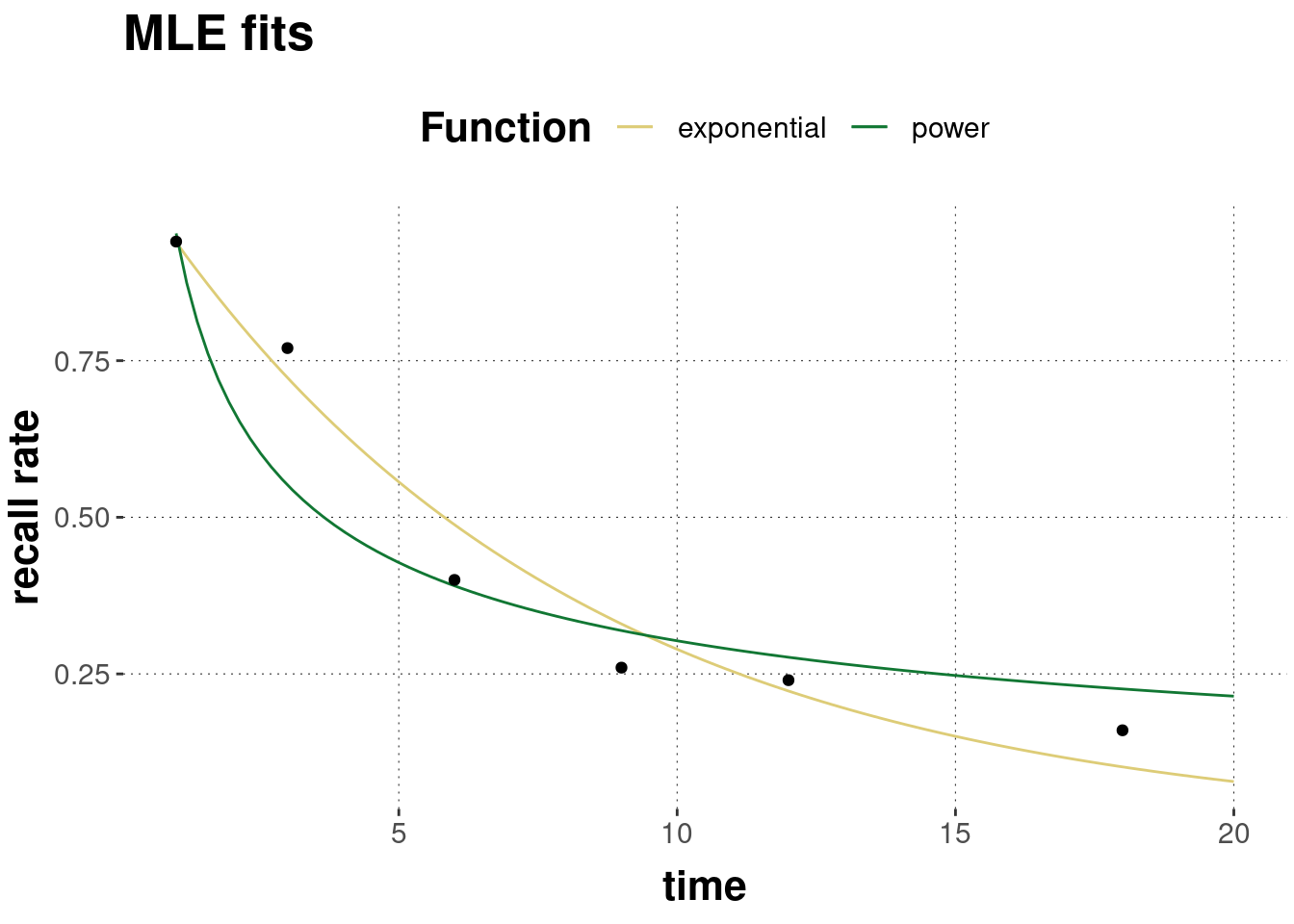
Figure 10.2: Predictions of the exponential and the power model under best-fitting parameter values.
By visual inspection of Figure 10.2 alone, it is impossible to say with confidence which model is better. Numbers might help see more fine-grained differences. So, let’s look at the log-likelihood and the corresponding probability of the data for each model under each model’s best fitting parameter values.
predExp <- expo(t, a, b)
predPow <- power(t, c, d)
modelStats <- tibble(
  model = c("expo", "power"),
  `log likelihood` = round(c(-bestExpo$value, -bestPow$value), 3),
  probability = signif(exp(c(-bestExpo$value, -bestPow$value)), 3),
  # sum of squared errors
  SS = round(c(sum((predExp - y)^2), sum((predPow - y)^2)), 3)
)
modelStats
## # A tibble: 2 × 4
## model `log likelihood` probability SS
## <chr> <dbl> <dbl> <dbl>
## 1 expo -18.7 7.82e- 9 0.019
## 2 power -26.7 2.47e-12 0.057The exponential model has a higher log-likelihood, a higher probability, and a lower sum of squares. This suggests that the exponential model is better.
The AIC-score of these models is a direct function of the negative log-likelihood. Since both models have the same number of parameters, we arrive at the same verdict as before: based on a comparison of AIC-scores, the exponential model is the better model.
get_AIC <- function(optim_fit) {
  2 * length(optim_fit$par) + 2 * optim_fit$value
}
AIC_scores <- tibble(
  AIC_exponential = get_AIC(bestExpo),
  AIC_power = get_AIC(bestPow)
)
AIC_scores
## # A tibble: 1 × 2
## AIC_exponential AIC_power
## <dbl> <dbl>
## 1 41.3 57.5How should we interpret the difference in AIC-scores? Some suggest that differences in AIC-scores larger than 10 should be treated as implying that the weaker model has practically no empirical support (Burnham and Anderson 2002). Adopting such a criterion, we would therefore favor the exponential model based on the data observed.
But we could also try to walk a more nuanced, more quantitative road. We would ideally want to know the absolute probability of \(M_i\) given the data: \(P(M_i \mid D)\). Unfortunately, to calculate this (by Bayes rule), we would need to normalize by quantifying over all models. Alternatively, we look at the relative probability of a small selection of models. Indeed, we can look at relative AIC-scores in terms of so-called Akaike weights (Wagenmakers and Farrell 2004; Burnham and Anderson 2002) to derive an approximation of \(P(M_i \mid D)\), at least for the case where we only consider a small set of candidate models. So, if we want to compare models \(M_1, \dots, M_n\) and \(\text{AIC}(M_i, D)\) is the AIC-score of model \(M_i\) for observed data \(D\), then the Akaike weight of model \(M_i\) is defined as:
\[ \begin{aligned} w_{\text{AIC}}(M_i, D) & = \frac{\exp (- 0.5 * \Delta_{\text{AIC}}(M_i,D) )} {\sum_{j=1}^k\exp (- 0.5 * \Delta_{\text{AIC}}(M_j,D) )}\, \ \ \ \ \text{where} \\ \Delta_{\text{AIC}}(M_i,D) & = \text{AIC}(M_i, D) - \min_j \text{AIC}(M_j, D) \end{aligned} \]
Akaike weights are relative and normalized measures, and may serve as an approximate measure of a model’s posterior probability given the data:
\[ P(M_i \mid D) \approx w_{\text{AIC}}(M_i, D) \]
For the running example at hand, this would mean that we could conclude that the posterior probability of the exponential model is approximately:
delta_AIC_power <- AIC_scores$AIC_power - AIC_scores$AIC_exponential
delta_AIC_exponential <- 0
Akaike_weight_exponential <- exp(-0.5 * delta_AIC_exponential) /
  (exp(-0.5 * delta_AIC_exponential) + exp(-0.5 * delta_AIC_power))
Akaike_weight_exponential
## [1] 0.9996841We can interpret this numerical result as indicating that, given a universe in which only the exponential and the power model exist, the posterior probability of the exponential model is almost 1 (assuming, implicitly, that both models are equally likely a priori). We would conclude from this approximate quantitative assessment that the empirical evidence supplied by the given data in favor of the exponential model is very strong.
Our approximation is better the more data we have. We will see a method below, the Bayesian method using Bayes factors, which computes \(P(M_i \mid D)\) in a non-approximate way.
Exercise 11.1
- Describe what the following variables represent in the AIC formula: \[ \begin{aligned} \text{AIC}(M_i, D_\text{obs}) & = 2k_i - 2\log P(D_\text{obs} \mid \hat{\theta_i}, M_i) \end{aligned} \]
- \(k_i\) stands for:
- \(\hat{\theta_i}\) stands for:
- \(P(D_\text{obs} \mid \hat{\theta_i}, M_i)\) stands for:
- Do you see that there is something “circular” in the definition of AICs? (Hint: What do we use the data \(D_{\text{obs}}\) for?)
We use the same data twice! We use \(D_{\text{obs}}\) to find the best fitting parameter values, and then we ask how likely \(D_{\text{obs}}\) is given the best fitting parameter values. If model comparison is about how well a model explains the data, then this is a rather circular measure: we quantify how well a model explains or predicts a data set after having “trained / optimized” the model for exactly this data set.
References
Burnham, Kenneth P., and David R. Anderson. 2002. Model Selection and Multimodel Inference: A Practical Information-Theoretic Approach. Berlin: Springer.
Wagenmakers, Eric-Jan, and Simon Farrell. 2004. “AIC Model Selection Using Akaike Weights.” Psychonomic Bulletin & Review 11 (1): 192–96.