Statement c. is correct.
17.5 Comparing Bayesian and frequentist estimates
As discussed in Chapter 9, parameter estimation is traditionally governed by two measures: (i) a point-estimate for the best parameter value, and (ii) an interval-estimate for a range of values that are considered “good enough”. Table 17.1 gives the most salient answers that the Bayesian and the frequentist approaches give.
| estimate | Bayesian | frequentist |
|---|---|---|
| best value | mean of posterior | maximum likelihood estimate |
| interval range | credible interval (HDI) | confidence interval |
For Bayesians, point-valued and interval-based estimates are just summary statistics to efficiently communicate about or reason with the main thing: the full posterior distribution. For the frequentist, the point-valued and interval-based estimates might be all there is. Computing a full posterior can be very hard. Computing point-estimates is usually much simpler. Yet, all the trouble of having to specify priors, and having to calculate a much more complex mathematical object, can pay off. An example which is intuitive enough is that of a likelihood function in a multi-dimensional parameter space where there is an infinite collection of parameter values that maximize the likelihood function (think of a plateau). Asking a godly oracle for “the” MLE can be disastrously misleading. The full posterior will show the quirkiness. In other words, to find an MLE can be an ill-posed problem where exploring the posterior surface is not.
Practical issues aside, there are also conceptual arguments that can be pinned against each other. Suppose you do not know the bias of a coin, you flip it once and it lands heads. The case in mathematical notation: \(k=1\), \(N=1\). As a frequentist, your “best” estimate of the coin’s bias is that it is 100% rigged: it will never land tails. As a Bayesian, with uninformed priors, your “best” estimate is, following Laplace rule, \(\frac{k+1}{N+2} = \frac{2}{3}\). Notice that there might be different notions of what counts as “best” in place. Still, the frequentist “best” estimate seems rather extreme.
What about interval-ranged estimates? Which is the better tool, confidence intervals or credible intervals? – This is hard to answer. Numerical simulations can help answer these questions.90 The idea is simple but immensely powerful. We simulate, repeatedly, a ground-truth and synthetic results for fictitious experiments, and then we apply the statistical tests/procedures to these fictitious data sets. Since we know the ground-truth, we can check which tests/procedures got it right.
Let’s look at a simulation set-up to compare credible intervals to confidence intervals, the latter of which are calculated by asymptotic approximation or the so-called exact method (see the info-box in Section 16.5). To do so, we repeatedly sample a ground-truth (e.g., a known coin bias \(\theta_{\text{true}}\)) from a flat distribution over \([0;1]\).91. We then simulate an experiment in a synthetic world with \(\theta_{\text{true}}\), using a fixed value of \(n\), here taken from the set \(n \in \left \{ 10, 25, 100, 1000 \right \}\). We then construct a confidence interval (either approximately or precisely) and a 95% credible interval; for each of the three interval estimates. We check whether the ground-truth \(\theta_{\text{true}}\) is not included in any given interval estimate. We calculate the mean number of times such as non-inclusion (errors!) happen for each kind of interval estimate. The code below implements this and the figure below shows the results based on 10,000 samples of \(\theta_{\text{true}}\).
# how many "true" thetas to sample
n_samples <- 10000
# sample a "true" theta
theta_true <- runif(n = n_samples)
# create data frame to store results in
results <- expand.grid(
  theta_true = theta_true,
  n_flips = c(10, 25, 100, 1000)
) %>%
  as_tibble() %>%
  mutate(
    outcome = 0,
    norm_approx = 0,
    exact = 0,
    Bayes_HDI = 0
  )

for (i in 1:nrow(results)) {

  # sample fictitious experimental outcome for current true theta
  results$outcome[i] <- rbinom(
    n = 1,
    size = results$n_flips[i],
    prob = results$theta_true[i]
  )

  # get CI based on asymptotic Gaussian
  norm_approx_CI <- binom::binom.confint(
    results$outcome[i],
    results$n_flips[i],
    method = "asymptotic"
  )
  results$norm_approx[i] <- !(
    norm_approx_CI$lower <= results$theta_true[i] &&
      norm_approx_CI$upper >= results$theta_true[i]
    )

  # get CI based on exact method
  exact_CI <- binom::binom.confint(
    results$outcome[i],
    results$n_flips[i],
    method = "exact"
  )
  results$exact[i] <- !(
    exact_CI$lower <= results$theta_true[i] &&
      exact_CI$upper >= results$theta_true[i]
  )

  # get 95% HDI (flat priors)
  Bayes_HDI <- binom::binom.bayes(
    results$outcome[i],
    results$n_flips[i],
    type = "highest",
    prior.shape1 = 1,
    prior.shape2 = 1
  )
  results$Bayes_HDI[i] <- !(
    Bayes_HDI$lower <= results$theta_true[i] &&
      Bayes_HDI$upper >= results$theta_true[i]
  )
}

results %>%
  gather(key = "method", "Type_1", norm_approx, exact, Bayes_HDI) %>%
  group_by(method, n_flips) %>%
  dplyr::summarize(avg_type_1 = mean(Type_1)) %>%
  ungroup() %>%
  mutate(
    method = factor(
      method,
      ordered = T,
      levels = c("norm_approx", "Bayes_HDI", "exact")
    )
  ) %>%
  ggplot(aes(x = as.factor(n_flips), y = avg_type_1, color = method)) +
  geom_point(size = 3) + geom_line(aes(group = method), size = 1.3) +
  xlab("number of flips per experiment") +
  ylab("proportion of exclusions of true theta")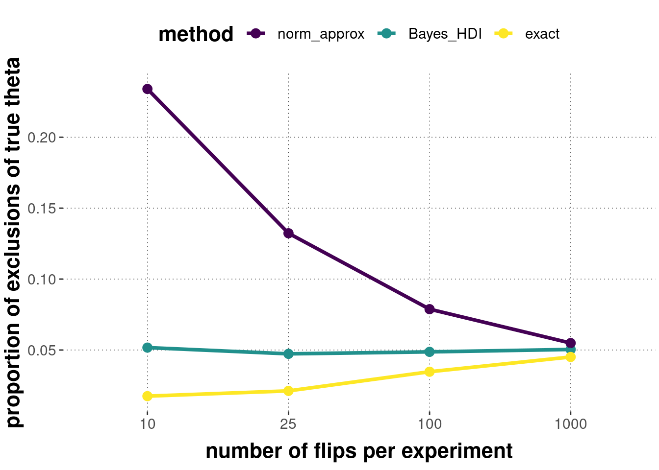
These results show a few interesting things. For one, looking at the error-level of the exact confidence intervals, we see that the \(\alpha\)-level of frequentist statistics is an upper bound on the amount of error. For a discrete sample space, the actual error rate can be substantially lower. Second, the approximate method for computing confidence intervals is off unless the sample size warrants the approximation. This stresses the importance of caring about when an approximation underlying a frequentist test is (not) warranted. Thirdly, the Bayesian credible interval has a “perfect match” to the assumed \(\alpha\)-level for all sample sizes. However, we must take into account that the simulation assumes that the Bayesian analysis “knows the true prior”. We have actually sampled the latent parameter \(\theta\) from a uniform distribution; and we have used a flat prior for the Bayesian calculations. Obviously, the more the prior divergences from the true distribution, and the fewer data observations we have, the more errors will the Bayesian approach make.
Exercise 9.5
Pick the correct answer:
The most frequently used point-estimate of Bayesian parameter estimation looks at…
…the median of the posterior distribution.
…the maximum likelihood estimate.
…the mean of the posterior distribution.
…the normalizing constant in Bayes rule.
The most frequently used interval-based estimate in frequentist approaches is…
…the support of the likelihood distribution.
…the confidence interval.
…the hypothesis interval.
…the 95% highest-density interval of the maximum likelihood estimate.
Statement b. is correct.