MLE is a special case of MAP with a uniform prior.
9.2 Point-valued and interval-ranged estimates
Let’s consider the “24/7” example with a flat prior again, concisely repeated in Figure 9.5.
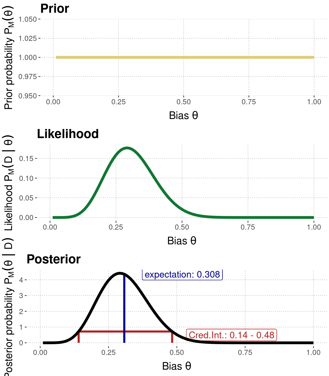
Figure 9.5: Prior (uninformative), likelihood and posterior for the 24/7 example.
The posterior probability distribution in Figure 9.5 contains rich information. It specifies how likely each value of \(\theta\) is, obtained by updating the original prior beliefs with the observed data. Such rich information is difficult to process and communicate in natural language. It is therefore convenient to have conventional means of summarizing the rich information carried in a probability distribution like in Figure 9.5. Customarily, we summarize in terms of a point-estimate and/or an interval estimate. The point estimate gives information about a “best value”, i.e., a salient point, and the interval estimate gives, usually, an indication of how closely other “good values” are scattered around the “best value”. The most frequently used Bayesian point estimate is the mean of the posterior distribution, and the most frequently used Bayesian interval estimate is the credible interval. We will introduce both below, alongside some alternatives (namely the maximum a posteriori, the maximum likelihood estimate and the inner-quantile range).
9.2.1 Point-valued estimates
A common Bayesian point estimate of parameter vector \(\theta\) is the mean of the posterior distribution over \(\theta\). It gives the value of \(\theta\) which we would expect to see when basing out expectations on the posterior distribution: \[ \begin{aligned} \mathbb{E}_{P(\theta \mid D)} = \int \theta \ P(\theta \mid D) \ \text{d}\theta \end{aligned} \] Taking the Binomial Model as example, if we start with flat beliefs, the expected value of \(\theta\) after \(k\) successes in \(N\) flips can be calculated rather easily as \(\frac{k+1}{n+2}\).49 For our example case, we calculate the expected value of \(\theta\) as \(\frac{8}{26} \approx 0.308\) (see also Figure 9.5).
Another salient point-estimate to summarize a Bayesian posterior distribution is the maximum a posteriori, or MAP, for short. The MAP is the parameter value (tuple) that maximizes the posterior distribution:
\[ \text{MAP}(P(\theta \mid D)) = \arg \max_\theta P(\theta \mid D) \]
While the mean of the posterior is “holistic” in the sense that it depends on the whole distribution, the MAP does not. The mean is therefore more faithful to the Bayesian ideal of taking the full posterior distribution into account. Moreover, depending on how Bayesian posteriors are computed/approximated, the estimation of a mean can be more reliable than that of a MAP.
The maximum likelihood estimate (MLE) is a point estimate based on the likelihood function alone. It specifies the value of \(\theta\) for which the observed data is most likely. We often use the notation \(\hat{\theta}\) to denote the MLE of \(\theta\):
\[ \begin{aligned} \hat{\theta} = \arg \max_{\theta} P(D \mid \theta) \end{aligned} \]
By ignoring the prior information entirely, the MLE is not a Bayesian notion, but a frequentist one (more on this in later chapters). For the binomial likelihood function, the maximum likelihood estimate is easy to calculate as \(\frac{k}{N}\), yielding \(\frac{7}{24} \approx 0.292\) for the running example. Figure 9.6 shows a graph of the non-normalized likelihood function and indicates the maximum likelihood estimate (the value that maximizes the curve).
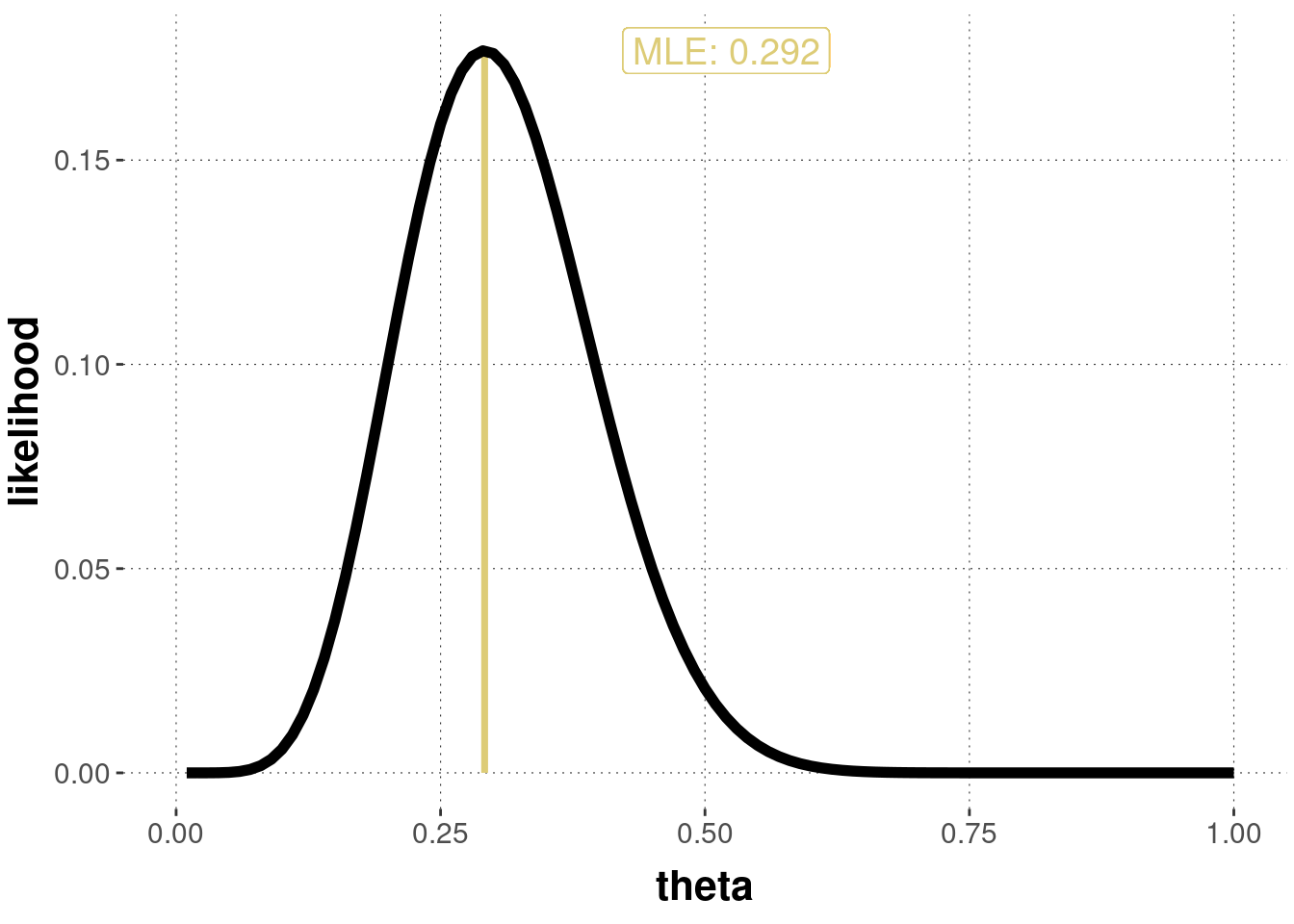
Figure 9.6: Non-normalized likelihood function for the observation of \(k=7\) successes in \(N=24\) flips, including maximum likelihood estimate.
Exercise 9.3
Can you think of a situation where MLE and MAP are the same? HINT: Think which prior eliminates the difference between them!
9.2.2 Interval-ranged estimates
A common Bayesian interval estimate of the coin bias parameter \(\theta\) is a credible interval.50 An interval \([l;u]\) is a \(\gamma\%\) credible interval for a random variable \(X\) if two conditions hold, namely \[ \begin{aligned} P(l \le X \le u) = \frac{\gamma}{100} \end{aligned} \] and, secondly, for every \(x \in[l;u]\) and \(x' \not \in[l;u]\) we have \(P(X=x) > P(X = x')\). Intuitively, a \(95\%\) credible interval gives the range of values in which we believe with relatively high certainty that the true value resides. Figure 9.5 indicates the \(95\%\) credible interval, based on the posterior distribution \(P(\theta \mid D)\) of \(\theta\), for the 24/7 example.51
Instead of credible intervals, sometimes posteriors are also summarized in terms of the \(\gamma\%\) inner-quantile region. This is the interval \([l;u]\) such that
\[P(l \le X) = P(X \le u) = 0.5 \cdot (1 - \frac{\gamma}{100})\]
For example, a 95% inner-quantile region contains all values except the smallest and largest values what each comprise 2.5% of the probability mass/density. The inner-quantile range is easier to compute and does not have trouble with multi-modality. This is why it is frequently used to approximate Bayesian credible intervals. However, care must be taken because the inner-quantile range is not as intuitive a measure of the “best values” as credible intervals. While credible intervals and inner quantile regions coincide for distributions with a symmetric distribution around a single maximum, and so tend to coincide for large sample size when posteriors tend to converge to normal distributions, there are cases of clear divergence. Figure 9.7 shows such a case. While the inner-quantile region does not include the most likely values, the credible interval does.
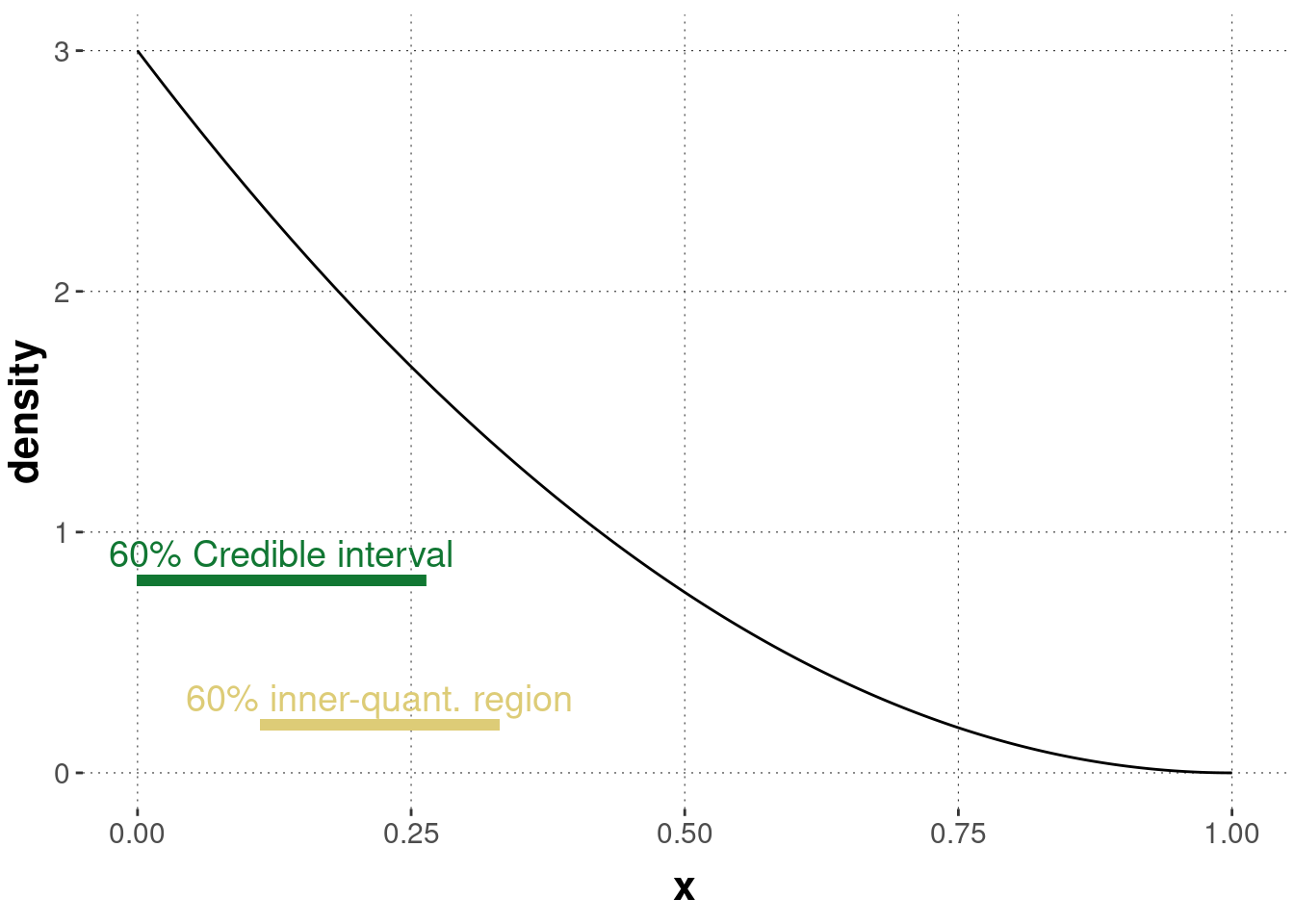
Figure 9.7: Difference between a 95% credible interval and a 95% inner-quantile region.
9.2.3 Computing Bayesian estimates
As mentioned, the most common (and arguably best) summaries to report for a Bayesian posterior are the posterior mean and a credible interval. The aida package which accompanies this book has a convenience function called aida::summarize_sample_vector() that gives the mean and 95% credible interval for a vector of samples.
You can use it like so:
# take samples from a posterior (24/7 example with flat priors)
posterior_samples <- rbeta(100000, 8, 18)
# get summaries
aida::summarize_sample_vector(
  # vector of samples
  samples = posterior_samples,
  # name of output column
  name = "theta"
)
## # A tibble: 1 × 4
## Parameter `|95%` mean `95%|`
## <chr> <dbl> <dbl> <dbl>
## 1 theta 0.145 0.308 0.4869.2.4 Excursion: Computing MLEs and MAPs in R
Computing the maximum or minimum of a function, such as an MLE or MAP estimate, is a common problem. R has a built-in function optim that is useful for finding the minimum of a function. (If a maximum is needed, just multiply by \(-1\) and search the minimum with optim.)
We can use the optim function to retrieve an MLE for 24/7 data and the Binomial Model (with flat priors) using conjugacy like so:
# perform optimization
MLE <- optim(
  # starting value for optimization
  par = 0.2,
  # funtion to minimize (= optimize)
  fn = function(par){
    -dbeta(par, 8, 18)
  },
  # method of optimization (for 1-d cases)
  method = "Brent",
  # lower and upper bound of possible parameter values
  lower = 0,
  upper = 1
)
# retrieve MLE
MLE$par
## [1] 0.2916667Indeed, the value obtained by computationally approximating the maximum likelihood estimate for this likelihood function coincides with the true value of \(\frac{7}{24}\).
This is also known as Laplace’s rule or the rule of succession.↩︎
Also frequently called “highest-density intervals”, even when we are dealing not with density but probability mass.↩︎
Not all random variables have a credible interval for a given \(\gamma\), according to this definition. A bimodal distribution might not, for example. A bi-modal distribution has two regions of high probability. We can, therefore, generalize the concept to a finite set of disjoint convex credible regions, all of which have the second property of the definition above and all of which conjointly are realized with \(\gamma\%\) probability. Unfortunately, common parlor uses the term “credible interval” to refer to credible regions as well. The same disaster occurs with alternative terms, such as “\(\gamma\%\) highest-density intervals”, which also often refers to what should better be called “highest-density regions”.↩︎