12.3 A Bayesian approach
The Bayesian approach to linear regression just builds on the likelihood-based approach of the last section, to which it adds priors for the model parameters \(\beta\) (a vector of regression coefficients) and \(\sigma\) (the standard deviation of the normal distribution).
The next Chapter 13 introduces ways of conveniently sampling from Bayesian regression models with variable specifications of these model priors using the R package brms.
This section introduces a Bayesian regression model with non-informative priors which extends the non-informative priors model for inferring the parameters of a normal distribution, which was introduced in section 9.4.
The Bayesian non-informative priors regression model uses the same likelihood function as the likelihood-based model from before and assumes essentially the same non-informative priors as the model from section 9.4. Concretely, it assumes an (improper) flat distribution over regression coefficients, and it assumes that the variance \(\sigma^2\) is log-uniformly distributed, which is equivalent to saying that \(\sigma^2\) follows an inverse distribution. So, for a regression problem with \(k\) predictors, predictor matrix \(X\) of size \(x \times (k+1)\) and dependent data \(y\) of size \(n\), we have:
\[ \begin{aligned} \beta_j & \sim \mathrm{Uniform}(-\infty, \infty) \ \ \ \text{for all } 0 \le j \le k \\ \log(\sigma^2) & \sim \mathrm{Uniform}(-\infty, \infty) \\ y_i & \sim \text{Normal}((X \beta)_i, \sigma) \end{aligned} \]
Using this prior, we can calculate a closed-form of the posterior to sample from (for details see Gelman et al. (2014) Chap. 14). The posterior has the general form:
\[ P(\beta, \sigma^2 \mid y) \propto P(\sigma^2 \mid y) \ P(\beta \mid \sigma^2, y) \]
Without going into details here, the posterior distribution of the variance \(\sigma^2\) is an inverse-\(\chi^2\):
\[ \sigma^2 \mid y \sim \text{Inv-}\chi^2(n-k, \color{gray}{\text{ some-complicated-term}}) \]
The posterior of the regression coefficients is a (multivariate) normal distribution:
\[ \beta \mid \sigma^2, y \sim \text{MV-Normal}(\hat{\beta}, \color{gray}{\text{ some-complicated-term}}) \] What is interesting to note is that the mean of the posterior distribution of regression coefficients is exactly the optimal solution for ordinary least-squares regression and the maximum likelihood estimate:
\[ \hat{\beta} = (X^T \ X)^{-1}\ X^Ty \]
This is not surprising given that the mean of a normal distribution is also its mode and that the MAP for a non-informative prior coincides with the MLE.
The aida package provides the convenience function aida::get_samples_regression_noninformative for sampling from the posterior of the Bayesian non-informative priors model. We use this function below but show it explicitly first:
get_samples_regression_noninformative <- function(
  X, # design matrix
  y, # dependent variable
  n_samples = 1000
)
{
  if(is.null(colnames(X))) {
    stop("Design matrix X must have meaningful column names for coefficients.")
  }
  n <- length(y)
  k <- ncol(X)

  # calculating the formula from Gelman et al
  # NB 'solve' computes the inverse of a matrix
  beta_hat <- solve(t(X) %*% X) %*% t(X) %*% y
  V_beta   <- solve(t(X) %*% X)

  # 'sample co-variance matrix'
  s_squared <- 1 / (n - k) * t(y - (X %*% beta_hat)) %*% (y - (X %*% beta_hat))

  # sample from posterior of variance
  samples_sigma_squared <- extraDistr::rinvchisq(
    n   = n_samples,
    nu  = n - k,
    tau = s_squared
  )

  # sample full joint posterior triples
  samples_posterior <- map_df(
    seq(n_samples),
    function(i) {
      s <- mvtnorm::rmvnorm(1, beta_hat, V_beta * samples_sigma_squared[i])
      colnames(s) = colnames(X)
      as_tibble(s) %>%
        mutate(sigma = samples_sigma_squared[i] %>% sqrt())
    }
  )
  return(samples_posterior)
}
Let’s apply this function to the running example of this chapter:
# variables for regression
y <- murder_data$murder_rate
x <- murder_data$unemployment

# the predictor 'intercept' is just a
# column vector of ones of the same length as y
int <- rep(1, length(y))

# create predictor matrix with values of all explanatory variables
#    (here only intercept and slope for MAD)
X <- matrix(c(int, x),  ncol = 2)
colnames(X) <- c("intercept", "slope")

# collect samples with convenience function
samples_Bayes_regression <- aida::get_samples_regression_noninformative(X, y, 10000)
The tibble samples_Bayes_regression contains 10,000 samples from the posterior. Let’s have a look at the first couple of samples:
head(samples_Bayes_regression)## # A tibble: 6 × 3
## intercept slope sigma
## <dbl> <dbl> <dbl>
## 1 -40.8 8.74 4.40
## 2 -26.1 6.70 6.03
## 3 -37.2 8.30 4.08
## 4 -30.1 7.09 7.03
## 5 -29.8 7.13 5.08
## 6 -22.3 6.14 5.05Remember that each sample is a triple, one value for each of the model’s parameters.
We can also look at some summary statistics, using another convenience function from the aida package:
rbind(
  aida::summarize_sample_vector(samples_Bayes_regression$intercept, "intercept"),
  aida::summarize_sample_vector(samples_Bayes_regression$slope, "slope"),
  aida::summarize_sample_vector(samples_Bayes_regression$sigma, "sigma")
)
## # A tibble: 3 × 4
## Parameter `|95%` mean `95%|`
## <chr> <dbl> <dbl> <dbl>
## 1 intercept -42.7 -28.5 -14.5
## 2 slope 5.08 7.08 9.07
## 3 sigma 3.59 5.32 7.15Here’s a density plot of the (marginal) posteriors for each parameter value:
samples_Bayes_regression %>%
  pivot_longer(cols = everything(), values_to = "sample", names_to = "parameter") %>%
  mutate(parameter = factor(parameter, levels = c('intercept', 'slope', 'sigma'))) %>%
  ggplot(aes(x = sample)) +
    geom_density(fill = "lightgray", alpha = 0.5) +
    facet_wrap(~parameter, scales = "free")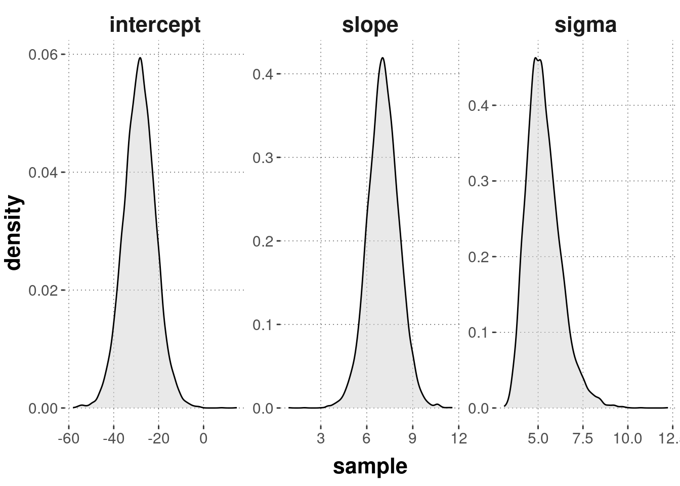
While these results are approximate, because they are affected by random sampling, they also convey a sense of uncertainty: given the data and the model, how certain should we be that, say, the slope is really at 7.08?
We could, for instance, now test the hypothesis that the factor unemployment does not contribute at all to predicting the value of the variable murder_rate.
This could be addressed as the point-valued hypothesis that the slope coefficient is exactly equal to zero.
Since the 95% credible interval clearly excludes this value, we might (based on this binary decision logic) now say that based on the model and the data there is reason to believe that unemployment does contribute to predicting murder_rate, in fact, that the higher a city’s unemployment rate, the higher we should expect its murder rate to be.
(Remember: this is not a claim about any kind of causal relation!)