11.1 Statistical hypotheses
Given a model \(M\) with parameter space \(\Theta\), a statistical hypothesis, in the sense entertained here, is an assumption (made for purposes of investigation) that certain parameters \(\Theta_i\) take on only a restricted range of values. For example, we might be interested in the question of whether a particular coin is fair. We consider the Binomial model, which contains the coin bias parameter \(\theta_c\). Informal assumptions about the coin’s bias can then be translated into a concrete question about values of \(\theta_{c}\).
This chapter considers three types of statistical hypotheses, which are also represented schematically in Figure 11.1. While all of the below also applies to discrete parameters and vectors of parameters, the implicit assumption in what follows is that we are dealing with a single continuous parameter.
- Point-valued hypotheses ask whether it is plausible that the parameter of relevance is identical to exactly one specific value. For example, in a Binomial model with the coin’s bias parameter \(\theta_{c}\), a point-valued hypothesis could be that \(\theta_c = 0.5\). More generally, we write \(\theta = \theta^*\) for a point-valued hypothesis about some (singular) parameter \(\theta\).
- ROPE-d hypotheses, where “ROPE” is short for region of practical equivalence, define a small \(\epsilon\)-region around a point-value of interest, and address the question of whether it is plausible that the parameter value lies inside this interval. For example, suppose that instead of addressing the point-valued hypothesis \(\theta_{c} = 0.5\) about a coin’s latent bias, we are able (e.g., through prior research or a priori conceptual considerations) to specify a reasonable region of practical equivalence (= ROPE) around the parameter value of interest. For instance, we might know that a difference of 0.1 in a coin’s bias really counts as normal slack and negligible for practical purposes. We then address the ROPE-d hypothesis that \(\theta_{c} \in [0.49, 0.51]\). More generally, we write \(\theta \in [\theta^* - \epsilon\ ;\ \theta^* + \epsilon]\), or \(\theta = \theta^* \pm \epsilon\) for ROPE-d hypothesis around the pivotal values \(\theta^*\).
- Directional hypotheses fix a specific parameter value, as a lower or upper bound and ask whether it is plausible that the parameter’s value is bigger or smaller than that fixed value. For example, \(\theta_{c} > 0.5\) could be the directional hypothesis that a coin is biased towards heads.
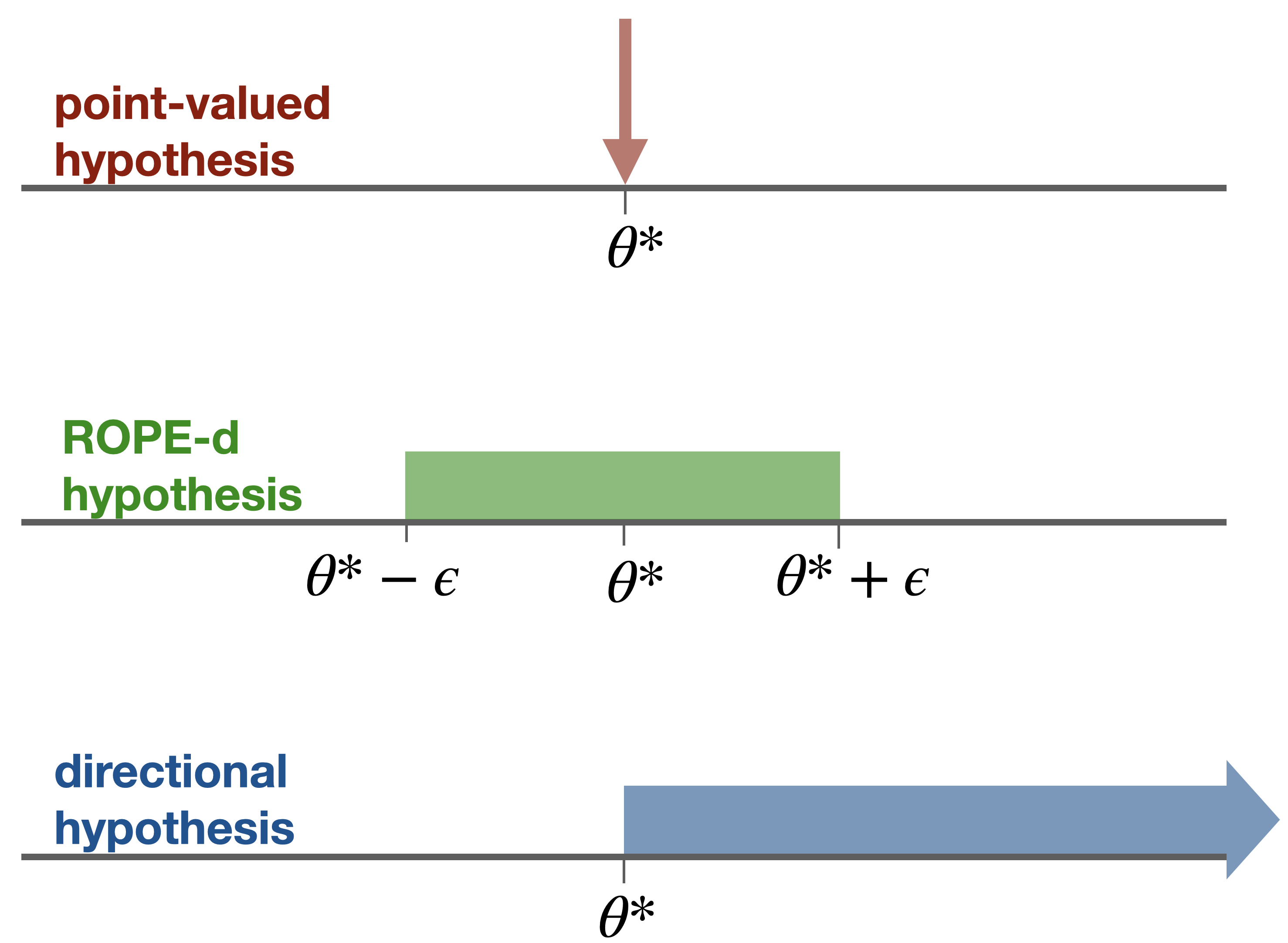
Figure 11.1: Three common types of hypotheses anchored to a point-value of interest of a parameter.
Ignoring trivial edge cases, both ROPE-d and directional hypotheses are instances of interval-based hypotheses in the sense that they assume that the true value lies in an interval.
The complement of a point-valued hypothesis \(\theta = \theta^*\) is the hypothesis that the true value is not equal to the critical value: \(\theta \neq \theta^*\). The complement of an interval-based hypothesis is the hypothesis that the true parameter value does not lie in the relevant interval. For example, the complement of the ROPE-d hypothesis \(\theta \in [\theta^* - \epsilon\ ;\ \theta^* + \epsilon]\) is that \(\theta \not \in [\theta^* - \epsilon\ ;\ \theta^* + \epsilon]\).
In the context of hypothesis testing, in particular frequentist testing (see Chapter 16), we often address the hypothesis to be tested as the null hypothesis. The complement of the null hypothesis is called alternative hypothesis.