Testing hypotheses based on parameter estimation, and in particular the categorical decision rules for accepting or rejecting hypotheses outlined in the previous section, only give a very coarse-grained picture.
Bayesian analysis is about providing quantitative information about uncertainty and evidence, which are intuitive and easily interpretable.
So, we would also like to have a quantitative assessment of the evidence for or against a hypothesis provided by some data against the background of a given model.
This is what the comparison-based approaches to Bayesian hypothesis testing give us.
Here is some further motivation why model comparison might be a good replacement for “testing via estimation”.
A statistical hypothesis \(H\) is basically an event: a subset of parameter values are picked out of the whole parameter space.
After observing data \(D_\text{obs}\) and based on model \(M\), the ideal measure to have is \(P_M(H \mid D_\text{obs})\): given data and model, how likely is the hypothesis in question?
The problem with this posterior formulation \(P_M(H \mid D_\text{obs})\) is that, for it to be meaningful, it must quantify over the set of all alternative hypotheses.
If \(H\) is a point-valued hypothesis over a single parameter, the set of all alternative hypotheses could comprise all other logically possible point-valued hypotheses for the same parameter.
But then, if that parameter is a continuous parameter, the posterior density at \(P_M(H \mid D_\text{obs})\) is not meaningfully interpretable as a probability (mass).
If \(H\) is an interval-based hypothesis, the posterior \(P_M(H \mid D_\text{obs})\) would be meaningfully interpretable as a probability (mass), but still the question of what exactly the space of alternatives is is left implicit.
Moreover, the posterior \(P_M(H \mid D_\text{obs})\) is influenced by the model’s prior over \(H\).
So, a nominally high value of \(P_M(H \mid D_\text{obs})\) is as such uninteresting because we would need to take the prior \(P_M(H)\) into account as well.
This is why a comparison-based approach to Bayesian hypothesis testing explicitly compares two models:
The null model\(M_0\) is the model that incorporates the assumption of the hypothesis \(H\) to be tested. For example, the null model would put prior probability zero on those parameter values which are ruled out by \(H\).
The alternative model\(M_1\) is an explicitly formulated model which incorporates some contextually or technically useful alternative to \(M_0\).
The comparison-based approach to hypothesis testing then quantifies, using Bayes factors, the evidence that \(D_\text{obs}\) provides for or against \(M_0\) (the model representing the “null hypothesis”) over the alternative model \(M_1\) (the model representing the alternative hypothesis).
In this way, by looking at the ratio:
this approach is independent of the prior probability assigned to models \(P(M_0)\) and \(P(M_1)\).
Notice, however, that it is not independent of the priors over \(\theta\) used in \(M_1\)!
When the null hypothesis is point-valued, the alternative model is not based on the complement \(\theta \neq \theta^*\), but on the technically much more practical and also conceptually more plausible alternative model that assumes that \(\theta\) is free to range over a larger interval including, but not limited to \(\theta^*\). We can then use the so-called Savage-Dickey method, described in Section 11.4.1, to compare the null and the alternative models as so-called nested models.
When the null hypothesis is interval-valued, the alternative model can be conceived as based on the complement of the null hypothesis. We can then use an extension of the Savage-Dickey method based on a so-called encompassing model, described in Section 11.4.2, where we construe both the null model and the alternative model as nested under a third, well, encompassing model.
This chapter shows how Bayes factors can be approximated based on samples from the posterior following both of these approaches.
11.4.1 The Savage-Dickey method
The Savage-Dickey method is a very convenient way of computing Bayes factors for nested models, especially when models only differ with respect to one parameter.
Suppose that there are \(n\) continuous parameters of interest \(\theta = \langle \theta_1, \dots, \theta_n \rangle\). \(M_1\) is a (Bayesian) model defined by \(P(\theta \mid M_1)\) and \(P(D \mid \theta, M_1)\). \(M_0\) is properly nested under \(M_1\) if:
Intuitively put, \(M_0\) is properly nested under \(M_1\), if \(M_0\) is a special case of \(M_1\) which fixes certain parameters to specific point-values.
Notice that the last condition is satisfied in particular when \(M_1\)’s prior over \(\theta_1, \dots, \theta_{i-1}\) is independent of the values for the remaining parameters.
We can express a point-valued hypothesis in terms of a model \(M_0\) which is nested under the alternative model \(M_1\), the latter of which assumes that the parameters in question can take more than one value.
For such properly nested models, we can compute a Bayes factor efficiently using the following result.
Theorem 11.1 (Savage-Dickey Bayes factors for nested models) Let \(M_0\) be properly nested under \(M_1\) s.t. \(M_0\) fixes \(\theta_i = x_i, \dots, \theta_n = x_n\). The Bayes factor \(\text{BF}_{01}\) in favor of \(M_0\) over \(M_1\) is then given by the ratio of posterior probability to prior probability of the parameters \(\theta_i = x_i, \dots, \theta_n = x_n\) from the point of view of the nesting model \(M_1\):
Proof. Let’s assume that \(M_0\) has parameters \(\theta = \langle\phi, \psi\rangle\) with \(\phi = \phi_0\), and that \(M_1\) has parameters \(\theta = \langle\phi, \psi \rangle\) with \(\phi\) free to vary. If \(M_0\) is properly nested under \(M_1\), we know that \(\lim_{\phi \rightarrow \phi_0} P(\psi \mid \phi, M_1) = P(\psi \mid M_0)\). We can then rewrite the marginal likelihood under \(M_0\) as follows:
The result follows if we divide by \(P(D \mid M_1)\) on both sides of the equation.
11.4.1.1 Example: 24/7
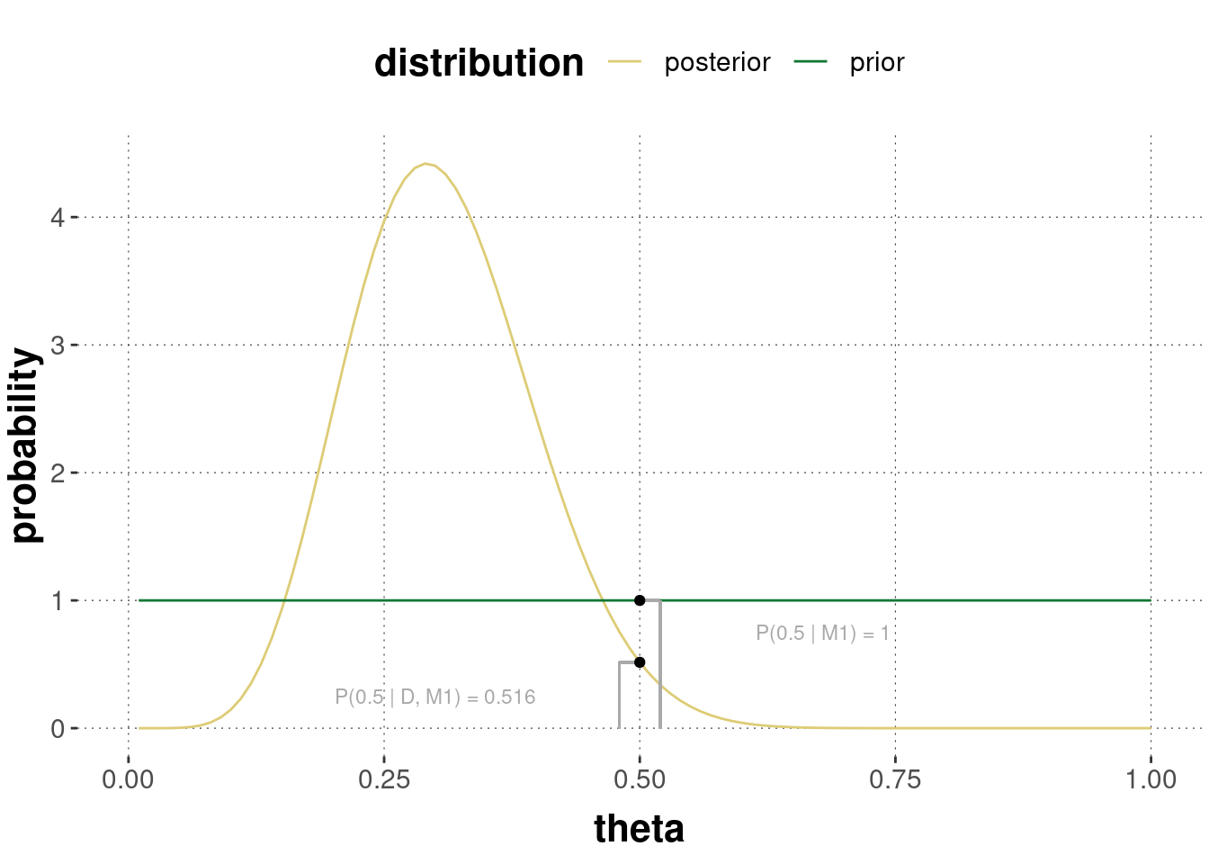
Here is an example based on the 24/7 data. For a nesting model with a flat prior (\(\theta \sim^{M_1} \text{Beta}(1,1)\)), and a point hypothesis \(\theta_c = 0.5\), we just have to calculate the prior and posterior probability of the critical value \(\theta_c = 0.5\):
# point-value of interesttheta_star <-0.5# posterior probability in nesting modelposterior_theta_star <-dbeta(theta_star, 8, 18)# prior probability in nesting modelprior_theta_star <-dbeta(theta_star, 1, 1)# Bayes factor (using Savage-Dickey)BF_01 <- posterior_theta_star / prior_theta_starBF_01
## [1] 0.5157351
This is very minor evidence in favor of the alternative model (Bayes factor \(\text{BF}_{10} \approx 1.94\)). We would not like to draw any (strong) categorical conclusions from this result regarding the question of whether the coin might be fair. Figure 11.6 also shows the relation between prior and posterior at the point-value of interest.
Figure 11.6: Illustration of the Savage-Dickey method of Bayes factor computation for the 24/7 case.
11.4.1.2 Example: Simon task
In the previous 24/7 example, using the Savage-Dickey method was particularly easy because we know a closed-form solution of the precise posterior, so that we could easily calculate the posterior for the critical value without further ado.
When this is not the case, like in the application to the Simon task data, we have to obtain an estimate for the posterior density at the critical value, here: \(\delta = 0\), from the posterior samples which we obtain from sampling, as we did earlier in this chapter (using Stan).
An approximate method for obtaining this value is implemented in the polspline package (using polynomial splines to approximate the posterior curve).
# extract the samples for the delta parameter# from the earlier Stan fitdelta_samples <- tidy_draws_tt2 %>%filter(Parameter =="delta") %>%pull(value)# estimating the posterior density at delta = 0 with polynomial splinesfit.posterior <- polspline::logspline(delta_samples)posterior_delta_null <- polspline::dlogspline(0, fit.posterior)# computing the prior density of the point-value of interest# [NB: the prior on delta was a standard normal]prior_delta_null <-dnorm(0, 0, 1) # compute BF via Savage-DickeyBF_delta_null = posterior_delta_null / prior_delta_nullBF_delta_null
## [1] 2.148062e-14
We conclude from this result that the data provide extremely strong evidence against the null model, which assumes that \(\delta = 0\), when compared to an alternative model \(M_1\), which assumes that \(\delta \sim \mathcal{N}(0,1)\) in the prior.
Exercise 11.3: Bayes factors with the Savage-Dickey method
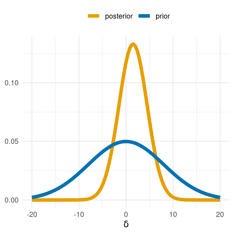
Look at the plot below. You see the prior distribution and the posterior distribution over the \(\delta\) parameter in a Bayesian \(t\)-test model. We are going to use this plot to determine (roughly) the Bayes factor of two models: the full Bayesian \(t\)-test model, and a model nested under this full model which assumes that \(\delta = 0\).
Describe in intuitive terms what it means for a Bayesian model to be nested under another model. It is sufficient to neglect the conditions on the priors.
A model nested under another model fixes certain parameters to specific values which may take on more than one value in the nesting model.
Write down the formula for the Bayes factor in favor of the null model (where \(\delta = 0\)) over the full model using the Savage-Dickey theorem.
Give a natural language paraphrase of the formula you wrote down above.
The Bayes factor in favor of the embedded null model over the embedding model is given by the posterior density at \(\delta = 0\) under the nesting model divided by the prior in the nesting model at \(\delta = 0\).
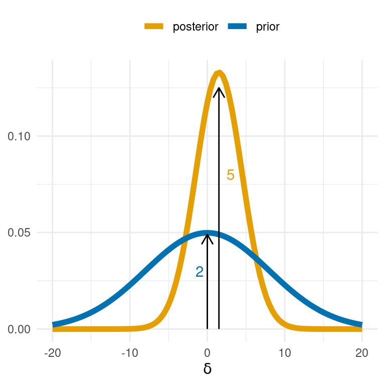
Now look at the plot above. Give your approximate guess of the Bayes factor in favor of the null model in terms of a fraction of whole integers (something like: \(\frac{4}{3}\) or \(\frac{27}{120}\), …).
\(BF_{01} \approx \frac{5}{2}\) (see plot above).
Formulate a conclusion to be drawn from this numerical result about the research hypothesis that the mean of the two groups compared here is identical. Write one concise sentence like you would in a research paper.
A BF of \(\frac{5}{2}\) is mild evidence in favor of the null model, but conventionally not considered strong enough to be particularly noteworthy.
11.4.1.3 [Excursion:] Calculating the Bayes factor precisely
under construction
11.4.2 Encompassing models
The Savage-Dickey method can be generalized to also cover interval-valued hypotheses.
The previous literature has focused on inequality-based intervals/hypotheses (like \(\theta \ge 0.5\)) (Klugkist, Kato, and Hoijtink 2005; Wetzels, Grasman, and Wagenmakers 2010; Oh 2014), but the method also applies to ROPE-d hypotheses.
The advantage of this method is that we can use samples from the posterior distribution to approximate integrals, which is more robust than having to estimate point-values of posterior density.
Following previous work (Klugkist, Kato, and Hoijtink 2005; Wetzels, Grasman, and Wagenmakers 2010; Oh 2014), the main idea is to use so-called encompassing priors. Let \(\theta\) be a single parameter of interest (for simplicity53), which can in principle take on any real value. We are interested in the interval-based hypotheses:
\(H_0 \colon \theta \in I_0\), and
\(H_1 \colon \theta \in I_{1}\)
where \(I_{0}\) is an interval, possibly half-open and \(I_1\) is the “negation” of \(I_0\) (in the sense that \(I_1 = \left \{ \theta \mid \theta \not \in I_0 \right \}\).
An encompassing model\(M_e\) has a suitable likelihood function \(P(D \mid \theta, \omega, M_{e})\) (where \(\omega\) is a vector of other parameters besides the parameter \(\theta\) of interest, so-called “nuisance parameters”).
It also defines a prior \(P(\theta, \omega \mid M_{e})\), which does not already rule out \(H_{0}\) or \(H_{1}\).
Generalizing over the Savage-Dickey approach, we construct two models, one for each hypothesis, both of which are nested under the encompassing model:
We assume that the priors over \(\theta\) are independent of the nuisance parameters \(\omega\).
Both \(M_0\) and \(M_1\) have the same likelihood function as \(M_e\).
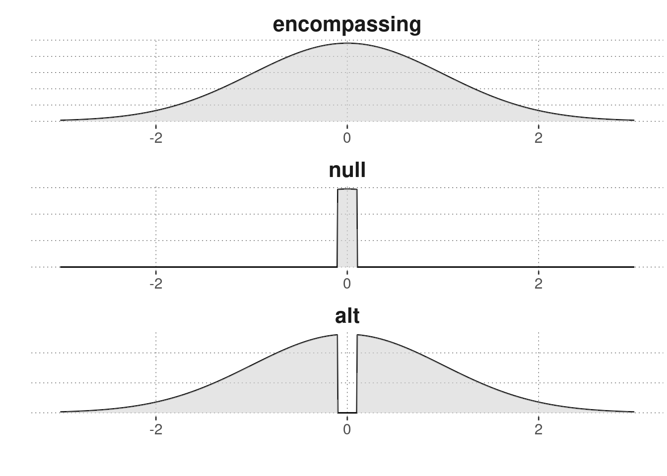
Figure 11.7 shows an example of the priors of an encompassing model for two nested models based on a ROPE-d hypothesis testing approach.
Figure 11.7: Example of the prior of an encompassing model and the priors of two models nested under it.
If our hypothesis of interest is \(I_0\), which is captured in \(M_0\), there are two comparisons we can make to quantify evidence in favor of or against \(M_0\): we can compare \(M_{0}\) against the encompassing model \(M_{e}\), or against its “negation” \(M_{1}\).
Bayes Factors for both comparisons can be easily expressed with the encompassing-models approach, as shown in Theorems 11.2 and 11.3.
Essentially, we can express Bayes Factors in terms of statements regarding the prior or posterior propability of \(I_0\) and \(I_1\) from the point of view of the encompassing model alone.
This means that we can approximate these Bayes Factors by just setting up one model, the encompassing model, and retrieving prior and posterior samples for it.
Concretely, Theorem 11.2 states that the Bayes Factor in favor of \(M_i\), when compared against the encompassing model \(M_e\) is the ratio of the posterior probability of \(\theta\) being in \(I_i\) divided by the prior probability, both from the perspective of \(M_e\).
Theorem 11.2 The Bayes Factor in favor of nested model \(M_{i}\) over encompassing model \(M_{e}\) is:
\[\begin{align*}
\mathrm{BF}_{ie} = \frac{P(\theta \in I_{i} \mid D, M_{e})}{P(\theta \in I_{i} \mid M_{e})}
\end{align*}\]
Proof. The following is only a sketch of a proof.
Important doemal details are glossed over.
For more detail, see (Klugkist and Hoijtink 2007).
We start by making three observations which hold for any model \(M_{i}\), \(i \in \left \{ 0,1 \right \}\), and any pair of vectors of parameter values \(\theta\prime, \omega\prime\) such that \(P(\theta\prime, \omega\prime \mid D, M_{i}) \neq 0\) (which entails that \(\theta\prime \in I_{I}\), \(P(\theta\prime, \omega\prime \mid M_{i}) > 0\) and \(P(D \mid \theta\prime, \omega\prime, M_{i}) > 0\)):
Observation 1: The definition of the posterior:
\[\begin{align*}
P(\theta\prime, \omega\prime \mid D, M_{i}) = \frac{P(D \mid \theta\prime, \omega\prime, M_{i}) \ P(\theta\prime, \omega\prime \mid M_{i})}{P(D \mid M_{i})}
\end{align*}\]
can be rewritten as:
\[\begin{align*}
P(D \mid M_{i}) = \frac{P(D \mid \theta\prime, \omega\prime, M_{i}) \ P(\theta\prime, \omega\prime \mid M_{i})}{P(\theta\prime, \omega\prime \mid D, M_{i})}
\end{align*}\]
This also holds for model \(M_{e}\).
Observation 2: The prior for \(\theta\prime, \omega\prime\) in \(M_{i}\) can be expressed in terms of the priors in \(M_{e}\) as:
\[\begin{align*}
P(\theta\prime, \omega\prime \mid M_{i}) = \frac{P(\theta\prime, \omega\prime \mid M_{e})}{P(\theta \in I_{i} \mid M_{e})}
\end{align*}\]
Observation 3: The posterior for \(\theta\prime, \omega\prime\) in \(M_{i}\) can be expressed in terms of the posteriors in \(M_{e}\) as:
\[\begin{align*}
P(\theta\prime, \omega\prime \mid D, M_{i}) = \frac{P(\theta\prime, \omega\prime \mid D, M_{e})}{P(\theta \in I_{i} \mid D, M_{e})}
\end{align*}\]
Theorem 11.2 states that the Bayes Factor in favor of \(M_0\), when compared against the alternative “negated” model \(M_1\) is the ratio of the posterior odds of \(\theta\) being in \(I_0\) divided by the prior odds, both from the perspective of \(M_e\).
Theorem 11.3 The Bayes Factor in favor of model \(M_{0}\) over alternative model \(M_{1}\) is:
\[\begin{align*}
\mathrm{BF}_{01} = \frac{P(\theta \in I_{0} \mid D, M_{e})}{P(\theta \in I_{1} \mid D, M_{e})} \ \frac{P(\theta \in I_{1} \mid M_{e})}{P(\theta \in I_{0} \mid M_{e})}
\end{align*}\]
Proof. This result follows as a direct corollary from Theorem 11.2 and Proposition 10.1.
Which comparison should be used for quantifying evidence in favor of or against \(M_0\): the encompassing model \(M_e\) or the alternative, “negation” model \(M_1\)?
There are good reasons for taking \(M_1\).
Here is why.
Suppose we hypothesize that a coin is biased towards heads, i.e., we consider the interval-valued hypothesis of interest \(H_0\) that \(\theta > 0.5\), where \(\theta\) is the parameter of a Binomial likelihood function.
Suppose we see \(k = 100\) from \(N=100\) tosses landing heads.
That is, intuitively, extremely strong evidence in favor of our hypothesis.
But if, as may be prudent, the encompassing model is neutral between our hypothesis and its negation, so that \(P(\theta > 0.5 \mid M_{e}) = 0.5\), the biggest Bayes Factor that we could possibly attain in favor of \(\theta > 0,5\) over the encompassing model, no matter what data we observe, is 2.
This is because, by Theorem 11.2, the numerator can at most be 1 and the denominator is fixed, by assumption, to be 0.5.
That does not seem like an intuitive way of quantifying the evidence in favor of \(\theta > 0.5\) when observing \(k=100\) out of \(N=100\), which seem quite overwhelming.
Instead, by Theorem 11.3, the Bayes Factor for a comparison of \(\theta > 0.5\) against \(\theta \le 0.5\) is virtually infinite, reflecting the intuition that this data set provides overwhelming support for the idea that \(\theta > 0.5\).
Based on considerations like these, it seems that the more intuitive comparison is against the negation of an interval-valued hypothesis, not against the encompassing model.
11.4.2.1 Example: 24/7
The Bayes factor using the ROPE-d method to compute the interval-valued hypothesis \(\theta = 0.5 \pm \epsilon\) is:
# set the scenetheta_null <-0.5epsilon <-0.01# epsilon margin for ROPEupper <- theta_null + epsilon # upper bound of ROPElower <- theta_null - epsilon # lower bound of ROPE# calculate prior odds of the ROPE-d hypothesisprior_of_hypothesis <-pbeta(upper, 1, 1) -pbeta(lower, 1, 1)prior_odds <- prior_of_hypothesis / (1- prior_of_hypothesis)# calculate posterior odds of the ROPE-d hypothesisposterior_of_hypothesis <-pbeta(upper, 8, 18) -pbeta(lower, 8, 18)posterior_odds <- posterior_of_hypothesis / (1- posterior_of_hypothesis)# calculate Bayes factorbf_ROPEd_hypothesis <- posterior_odds / prior_oddsbf_ROPEd_hypothesis
## [1] 0.5133012
This is unnoteworthy evidence in favor of the alternative hypothesis (Bayes factor \(\text{BF}_{10} \approx 1.95\)).
Notice that the reason why the alternative hypothesis does not fare better in this analysis is because it also includes a lot of parameter values (\(\theta > 0.5\)) which explain the observed data even more poorly than the values included in the null hypothesis.
We can also use this approach to test the directional hypothesis that \(\theta < 0.5\).
# calculate prior odds of the ROPE-d hypothesis# [trivial in the case at hand, but just to be explicit]prior_of_hypothesis <-pbeta(0.5, 1, 1) prior_odds <- prior_of_hypothesis / (1- prior_of_hypothesis)# calculate posterior odds of the ROPE-d hypothesisposterior_of_hypothesis <-pbeta(0.5, 8, 18)posterior_odds <- posterior_of_hypothesis / (1- posterior_of_hypothesis)# calculate Bayes factorbf_directional_hypothesis <- posterior_odds / prior_oddsbf_directional_hypothesis
## [1] 45.20512
Here we should conclude that the data provide substantial evidence in favor of the assumption that the coin is biased towards tails, when compared against the alternative assumption that it is biased towards heads.
If the dichotomy is “heads bias vs tails bias” the data clearly tilts our beliefs towards the “tails bias” possibility.
11.4.2.2 Example: Simon task
Using posterior samples, we can also do similar calculations for the Simon task.
Let’s first approximate the Bayes factor in favor of the ROPE-d hypothesis \(\delta = 0 \pm 0.1\) when compared against the alternative hypothesis \(\delta \not \in 0 \pm 0.1\).
# estimating the BF for ROPE-d hypothesis with encompassing priorsdelta_null <-0epsilon <-0.1# epsilon margin for ROPEupper <- delta_null + epsilon # upper bound of ROPElower <- delta_null - epsilon # lower bound of ROPE# calculate prior odds of the ROPE-d hypothesisprior_of_hypothesis <-pnorm(upper, 0, 1) -pnorm(lower, 0, 1)prior_odds <- prior_of_hypothesis / (1- prior_of_hypothesis)# calculate posterior odds of the ROPE-d hypothesisposterior_of_hypothesis <-mean( lower <= delta_samples & delta_samples <= upper )posterior_odds <- posterior_of_hypothesis / (1- posterior_of_hypothesis)# calculate Bayes factorbf_ROPEd_hypothesis <- posterior_odds / prior_oddsbf_ROPEd_hypothesis
## [1] 0
This is overwhelming evidence against the ROPE-d hypothesis that \(\delta = 0 \pm 0.1\).
We can also use this approach to test the directional hypothesis that \(\delta > 0.5\).
# calculate prior odds of the ROPE-d hypothesis# [trivial in the case at hand, but just to be explicit]prior_of_hypothesis <-1-pnorm(0, 0, 1)prior_odds <- prior_of_hypothesis / (1- prior_of_hypothesis)# calculate posterior odds of the ROPE-d hypothesisposterior_of_hypothesis <-mean( delta_samples >=0.5 )posterior_odds <- posterior_of_hypothesis / (1- posterior_of_hypothesis)# calculate Bayes factorbf_directional_hypothesis <- posterior_odds / prior_oddsbf_directional_hypothesis
## [1] Inf
Modulo imprecision induced by sampling, we see that the evidence in favor of the directional hypothesis \(\delta > 0.5\) is immense.
Exercise 11.4: True or False?
Decide for the following statements whether they are true or false.
An encompassing model for addressing ROPE-d hypotheses needs two competing models nested under it.
A Bayes factor of \(BF_{01} = 20\) constitutes strong evidence in favor of the alternative hypothesis.
A Bayes factor of \(BF_{10} = 20\) constitutes minor evidence in favor of the alternative hypothesis.
We can compute the BF in favor of the alternative hypothesis with \(BF_{10} = \frac{1}{BF_{01}}\).
Statements a. and d. are correct.
References
Klugkist, Irene, and Herbert Hoijtink. 2007. “The Bayes Factor for Inequality and about Equality Constrained Models.”Computational Statistics and Data Analysis 51 (12): 6367–79.
Klugkist, Irene, Bernet Kato, and Herbert Hoijtink. 2005. “Bayesian Model Selection Using Encompassing Priors.”Statistica Neelandica 59 (1): 57–69.
Oh, Man-Suk. 2014. “Bayesian Comparison of Models with Inequality and Equality Constraints.”Statistics and Probability Letters 84: 176–82.
Wetzels, Ruud, Raoul P. P. P. Grasman, and Eric-Jan Wagenmakers. 2010. “An Encompassing Prior Generalization of the Savage–Dickey Density Ratio.”Computational Statistics and Data Analysis 54: 2094–2102.
This method also works for vectors of parameters.↩︎