8.2 Notation & graphical representation
If it is important to communicate the assumptions underlying a statistical argument, and if models are means of making these assumptions formally explicit, then it follows that efficient communication of models is important too. We here follow the common practice of representing models using a special purpose formulaic notation and, where useful, a graph-based visual display in which probabilistic dependencies are lucidly represented.
Recall that the Binomial Model has a binomial likelihood function:
\[ P_M(k \mid \theta_c, N) = \text{Binomial}(k, N, \theta_c) = \binom{N}{k}\theta_c^k(1-\theta_c)^{N-k} \]
And a Beta distribution as a prior, e.g., with shape parameters set so that all values of \(\theta_c\) are equally likely.
\[ P_M(\theta_c) = \text{Beta}(\theta_c, 1, 1) \]
8.2.1 Formula notation
To concisely represent models, we use a special notation, which is very intuitive when we think about sampling. Instead of the above notation for the prior we write:
\[ \theta_c \sim \text{Beta}(1,1) \]
The symbol “\(\sim\)” is often read as “is distributed as”. You can also think of it as meaning that \(\theta_c\) is sampled from a \(\text{Beta}(1,1)\) distribution.
Similarly, for the likelihood function, we just write:
\[k \sim \text{Binomial}(\theta_c, N).\]
8.2.2 Graphical notation
When models get very complex and incorporate many parameters, it can be difficult to tease out the relations between all of the model’s components. In such a situation a graphical notation of a model is helpful. We here adopt the conventions described by Lee and Wagenmakers (2014). We represent every relevant variable as a node in a directed acyclic graph structure (a probabilistic network). The graph structure is used to indicate dependencies between the variables, with children depending on their parents. In visualizing this, we use the following general conventions:
- known or unknown (= latent) variable
- shaded nodes: observed variables
- unshaded nodes: unobserved / latent variables
- kind of variable:
- circular nodes: continuous variables
- square nodes: discrete variables
- kind of dependency:
- single line: stochastic dependency
- double line: deterministic dependency
For the Binomial Model this results in the relevant variables:
- number of trials (\(N\))
- number of success (\(k\))
- probability for success (\(\theta_c\))
Of these, \(N\) and \(k\) are observed and discrete variables, and \(\theta_c\) is a latent continuous variable. Clearly, the number of heads \(k\) depends on the coin bias \(\theta_c\) as well as on the number of trials \(N\). This yields a graphical and formulaic notation as in Figure 8.1.
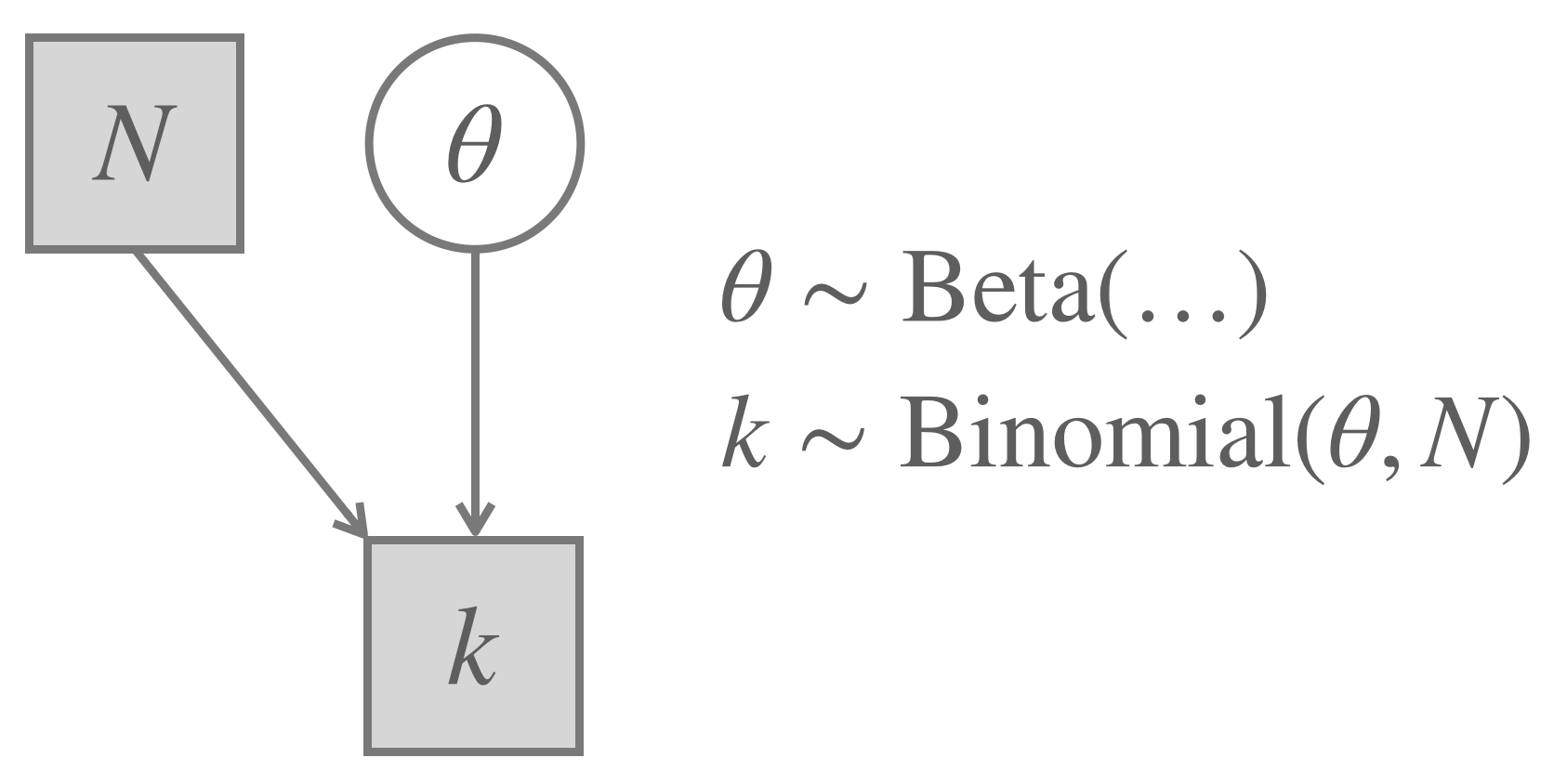
Figure 8.1: The Binomial Model. Notice that any specific Beta prior shape would yield what we here call a Binomial Model, which is why there are no concrete shape parameters given in this graph.