16.2 Quantifying evidence against a null-model with p-values

All prominent frequentist approaches to statistical hypothesis testing (see Section 16.1) agree that if empirical observations are sufficiently unlikely from the point of view of the null hypothesis $H_0$, this should be treated (in some way or other) as evidence against the null hypothesis. A measure of how unlikely the data is in the light of $H_0$ is the $p$-value.⁷³ To preview the main definition and intuition (to be worked out in detail hereafter), let’s first consider a verbal and then a mathematical formulation.

Definition $p$-value. The $p$-value associated with observed data $D_\text{obs}$ gives the probability, derived from the assumption that $H_0$ is true, of observing an outcome for the chosen test statistic that is at least as extreme evidence against $H_0$ as the observed outcome.

Formally, the $p$-value of observed data $D_\text{obs}$ is: \[ p\left(D_{\text{obs}}\right) = P\left(T^{|H_0} \succeq^{H_{0,a}} t\left(D_{\text{obs}}\right)\right) % = P(\mathcal{D}^{|H_0} \in \{D \mid t(D) \ge t(D_{\text{obs}})\}) \] where $t \colon \mathcal{D} \rightarrow \mathbb{R}$ is a test statistic which picks out a relevant summary statistic of each potential data observation, $T^{|H_0}$ is the sampling distribution, namely the random variable derived from test statistic $t$ and the assumption that $H_0$ is true, and $\succeq^{H_{0,a}}$ is a linear order on the image of $t$ such that $t(D_1) \succeq^{H_{0,a}} t(D_2)$ expresses that test value $t(D_1)$ is at least as extreme evidence against $H_0$ as test value $t(D_2)$ when compared to an alternative hypothesis $H_a$.⁷⁴

A few aspects of this definition are particularly important (and subsequent text is dedicated to making these aspects more comprehensible):

this is a frequentist approach in the sense that probabilities are entirely based on (hypothetical) repetitions of the assumed data-generating process, which assumes that $H_0$ is true;
the test statistic t plays a fundamental role and should be chosen such that:
- it must necessarily select exactly those aspects of the data that matter to our research question,
- it should optimally make it possible to derive a closed-form (approximation) of $T$,⁷⁵ and
- it would be desirable (but not necessary) to formulate $t$ in such a way that the comparison relation $\succeq^{H_{0,a}}$ coincides with a simple comparison of numbers: $t(D_1) \succeq^{H_{0,a}} t(D_2)$ iff $t(D_1) \ge t(D_2)$;
there is an assumed data-generating model buried inside notation $T^{|H_0}$; and
the notion of “more extreme evidence against $H_0$”, captured in comparison relation $\succeq^{H_{0,a}}$ depends on our epistemic purposes, i.e., what research question we are ultimately interested in.⁷⁶

The remainder of this section will elaborate on all of these points. It is important to mention that especially the third aspect (that there is an implicit data-generating model “inside of” classical hypothesis tests) is not something that receives a lot of emphasis in traditional statistics textbooks. Many textbooks do not even mention the assumptions implicit in a given test. Here we will not only stress key assumptions behind a test but present all of the assumptions behind classical tests in a graphical model, similar to what we did for Bayesian models. This arguably makes all implicit assumptions maximally transparent in a concise and lucid representation. It will also help see parallels between Bayesian and frequentist approaches, thereby helping to see both as more of the same rather than as something completely different. In order to cash in this model-based approach, the following sections will therefore introduce new graphical tools to communicate the data-generating model implicit in the classical tests we cover.

16.2.1 Frequentist null-models

We start with the Binomial Model because it is the simplest and perhaps most intuitive case. We work out what a $p$-value is for data for this model and introduce the new graphical language to communicate “frequentist models” in the following. We also introduce the notions of test statistic and sampling distribution based on a case that should be very intuitive, if not familiar.

The Binomial Model was covered before from a Bayesian point of view, where we represented it using graphical notation like in Figure 16.2 (repeated from before). Remember that this is a model to draw inferences about a coin’s bias $\theta$ based on observations of outcomes of flips of that coin. The Bayesian modeling approach treated the number of observed heads $k$ and the number of flips in total $N$ as given, and the coin’s bias parameter $\theta$ as latent.

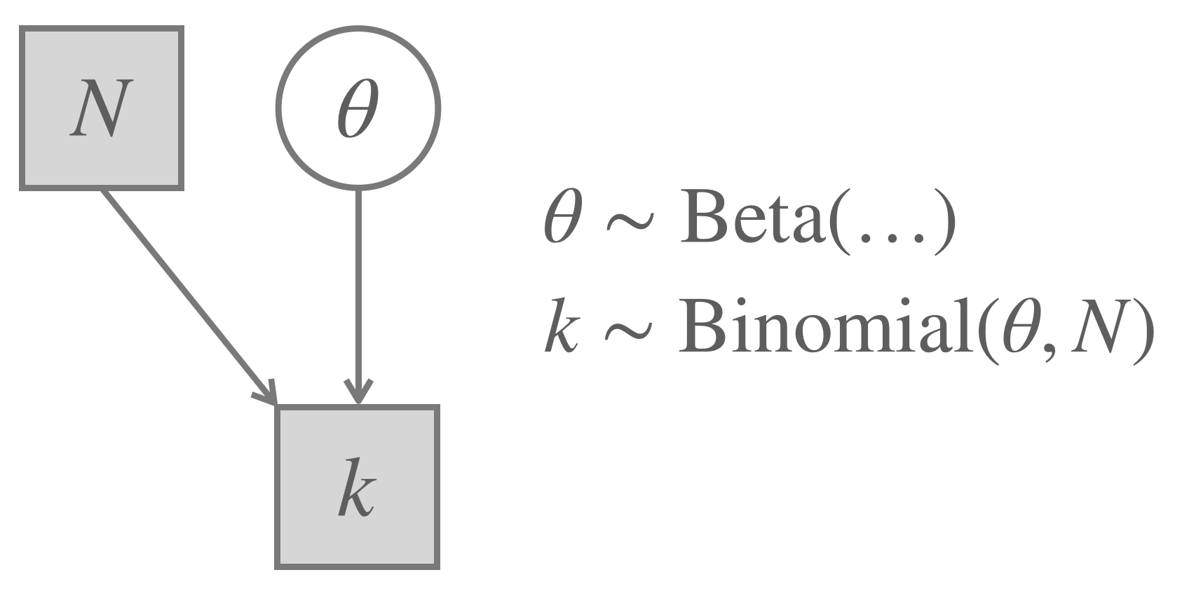
Figure 16.2: The Binomial Model (repeated from before) for a Bayesian approach to parameter inference/testing.

Actually, this way of writing the Binomial Model is a shortcut. It glosses over each individual data observation (whether the $i$-th coin flip was heads or tails) and jumps directly to the most relevant summary statistic of how many of the $N$ flips were heads. This might, of course, be just the relevant level of analysis. If our assumption is true that the outcome of each coin flip is independent of any other flip, and given our goal to learn something about $\theta$, all that really matters is $k$. But we can also rewrite the Bayesian model from Figure 16.2 as the equivalent extended model in Figure 16.3. In the latter representation, the individual outcomes of each flip are represented as $x_i \in \{0,1\}$. Each individual outcome is sampled from a Bernoulli distribution. Based on the whole vector of $x_i$-s and our knowledge of $N$, we derive the test statistic $k$, which maps each observation (a vector $x$ of zeros and ones) to a single number $k$ (the number of heads in the vector). Notice that the node for $k$ has a solid double edge, indicating that it follows deterministically from its parent nodes. This is why we can think of $k$ as a sample from a random variable constructed from “raw data” observations $x$.

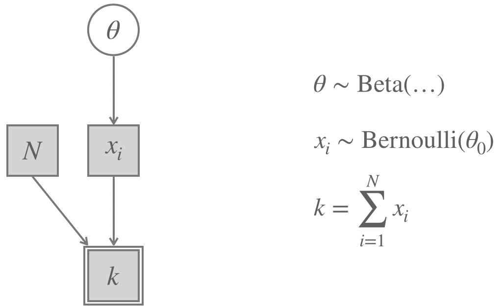
Figure 16.3: The Binomial Model for a Bayesian approach, extended to show ‘raw observations’ and the ‘summary statistic’ implicitly used.

Compare this latter representation in Figure 16.3 with the frequentist Binomial Model in Figure 16.4. The frequentist model treats the number of observations $N$ as observed, just like the Bayesian model. But it also fixes a specific value for the coin’s bias $\theta$. This is where the (point-valued) null hypothesis comes in. For purposes of analysis, we fix the value of the relevant unobservable latent parameter to a specific value (because we do not want to assign probabilities to latent parameters, but we still like to talk about probabilities somehow). In our graphical model in Figure 16.4, the node for the coin’s bias is shaded (= treated as known) but also has a dotted second edge to indicate that this is where our null hypothesis assumption kicks in. We then treat the data vector $x$ and, with it, the associated test statistic $k$ as unobserved. The data we actually observed will, of course, come in at some point. But the frequentist model leaves the observed data out at first in order to bring in the kinds of probabilities frequentist approaches feel comfortable with: probabilities derived from (hypothetical) repetitions of chance events. So, the frequentist model can now make statements about the likelihood of (raw) data $x$ and values of the derived summary statistic $k$ based on the assumption that the null hypothesis is true. Indeed, for the case at hand, we already know that the sampling distribution, i.e., the distribution of values for $k$ given $\theta_0$ is the Binomial distribution.

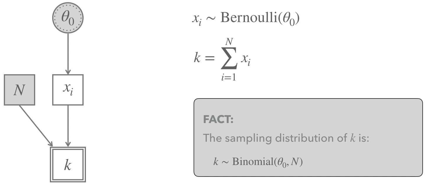
Figure 16.4: The Binomial Model for a frequentist binomial test.

Let’s take a step back. The frequentist model for the binomial case considers (“raw”) data of the form $\langle x_1, \dots, x_N \rangle$ where each $x_i \in \{0,1\}$ indicates whether the $i$-th flip was a success (= heads, = 1) or a failure (= tails, = 0). We identify the set of all binary vectors of length $N$ as the set of hypothetical data that we could, in principle, observe in a fictitious repetition of this data-generating process. $\mathcal{D}^{|H_0}$ is then the random variable that assigns each potential observation $D = \langle x_1, \dots, x_N \rangle$ the probability with which it would occur if $H_0$ (= a specific value of $\theta$) is true. In our case, that is:

\[P(\mathcal{D}^{|H_0} = \langle x_1, \dots, x_N \rangle) = \prod_{i=1}^N \text{Bernoulli}(x_i, \theta_0)\]

The model does not work with this raw data and its implied distribution (represented by random variable $\mathcal{D}^{|H_0}$), it instead uses a (very natural!) test statistic $t \colon \langle x_1, \dots, x_N \rangle \mapsto \sum_{i=1}^N x_i$. The sampling distribution for this model is therefore the distribution of values for the derived measure $k$ - a distribution that follows from the distribution of the raw data ($\mathcal{D}^{|H_0}$) and this particular test statistic $t$. In its most general form, we write the sampling distribution as $T^{|H_0} = t(\mathcal{D^{H_0}})$. ⁷⁷ It just so happens (what a relief!) that we know how to express $T^{|H_0}$ in a mathematically very concise fashion. It’s just the Binomial distribution, so that $k \sim \text{Binomial}(\theta_0, N)$. (Notice how the sampling distribution is really a function of $\theta_0$, i.e., the null hypothesis, and also of $N$.)

16.2.2 One- vs. two-sided $p$-values

After seeing a frequentist null model and learning about notions like “test statistic” and “sampling distribution”, let’s explore what a $p$-value is based on the frequentist Binomial Model. Our running example will be the 24/7 case, where $N = 24$ and $k = 7$. Notice that we are glossing over the “raw” data immediately and work with the value of the test statistic of the observed data directly: $t(D_{\text{obs}}) = 7$.

Remember that, by the definition given above, $p(D_{\text{obs}})$ is the probability of observing a value of the test statistic that is at least as extreme evidence against $H_0$ as $t(D_{\text{obs}})$, under the assumption that $H_0$ is true:

\[ p(D_{\text{obs}}) = P(T^{|H_0} \succeq^{H_{0,a}} t(D_{\text{obs}})) % = P(\mathcal{D}^{|H_0} \in \{D \mid t(D) \ge t(D_{\text{obs}})\}) \]

To fill this with life, we need to set a null hypothesis, i.e., a value $\theta_0$ of coin bias $\theta$, that we would like to collect evidence against. A fixed $H_0$ will directly fix $T^{|H_0}$, but we will have to put extra thought into how to conceptualize $\succeq^{H_{0,a}}$ for any given $H_0$. To make exactly this clearer is the job of this section. Specifically, we will look at what is standardly called a two-sided $p$-value and a one-sided $p$-value. The difference lies in whether we are testing a point-valued or an interval-based null hypothesis. So, let’s suppose that we want to test the following null hypotheses:

Is the coin fair ($\theta = 0.5$)?
Is the coin biased towards heads ($\theta > 0.5$)?

In the case of testing for fairness ($\theta = 0.5$), the pair of null hypothesis and alternative hypothesis are:

\[ \begin{aligned} H_0 \colon \theta = 0.5 && H_a \colon \theta \neq 0.5 \end{aligned} \]

The case for testing the null hypothesis $\theta > 0.5$ is slightly more convoluted. The frequentist construction of a null model strictly requires point-valued assumptions about all model parameters. Otherwise, subjective priors would sneak it. (NB: Even the assumption of equal probability of parameter values, as in a non-informative prior, is a biased and subjective assumption, according to frequentism.) We therefore actually test the point-valued null hypothesis $\theta = 0.5$, but we contrast it with a different alternative hypothesis, which is now one-sided:

\[ \begin{aligned} H_0 \colon \theta = 0.5 && H_a \colon \theta < 0.5 \end{aligned} \]

Case $\theta = 0.5$. To begin with, assume that we want to address the question of whether the coin is fair. Figure 16.5 shows the sampling distribution of the test statistic $k$. The probability of the observed value of the sampling statistic is shown in red.

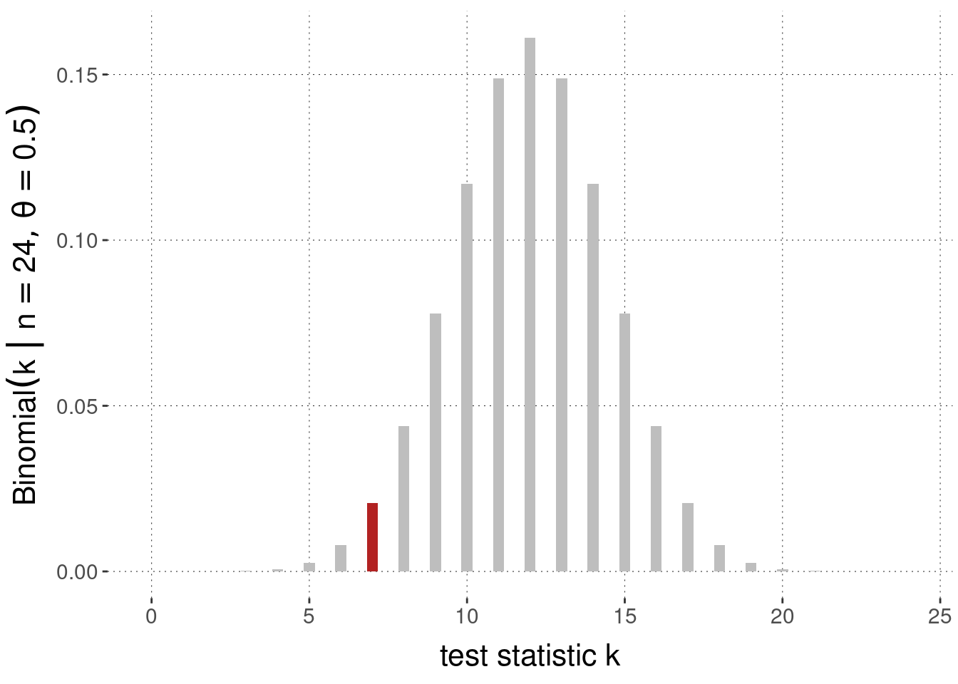
$Sampling distribution (here: Binomial distribution) and the probability associated with observed data $k=7$ highlighted in red, for $N = 24$ coin flips, under the assumption of a null hypothesis $\theta = 0.5$.$

Figure 16.5: Sampling distribution (here: Binomial distribution) and the probability associated with observed data $k=7$ highlighted in red, for $N = 24$ coin flips, under the assumption of a null hypothesis $\theta = 0.5$.

The question we need to settle to obtain a $p$-value is how to interpret $\succeq^{H_{0,a}}$ for this case. To do this, we need to decide which alternative values of $k$ would count as equally or more extreme evidence against the chosen null hypothesis when compared to the specified alternative hypothesis. The obvious approach is to use the probability of any value of the test statistic $k$ directly and say that observing $D_1$ counts as at least as extreme evidence against $H_0$ as observing $D_2$, $t(D_1) \succeq^{H_{0,a}} t(D_2)$, iff the probability of observing the test statistic associated with $D_1$ is at least as unlikely as observing $D_2$: $P(T^{|H_0} = t(D_1)) \le P(T^{|H_0} = t(D_2))$. To calculate the $p$-value in this way, we therefore need to sum up the probabilities of all values $k$ under the Binomial distribution (with parameters $N=24$ and $\theta = \theta_0 = 0.5$) that are no larger than the value of the observed $k = 7$. In mathematical language:⁷⁸

\[ p(k) = \sum_{k' = 0}^{N} [\text{Binomial}(k', N, \theta_0) <= \text{Binomial}(k, N, \theta_0)] \ \text{Binomial}(k', N, \theta_0) \]

In code, we calculate this $p$-value as follows:

# exact p-value for k = 7 with N = 24 and null hypothesis theta = 0.5
k_obs <- 7
N <- 24
theta_0 <- 0.5
tibble( lh = dbinom(0:N, N, theta_0) ) %>% 
  filter( lh <=  dbinom(k_obs, N, theta_0) ) %>% 
  pull(lh) %>% sum %>% round(5)

## [1] 0.06391

Figure 16.6 shows the values that need to be summed over in red.

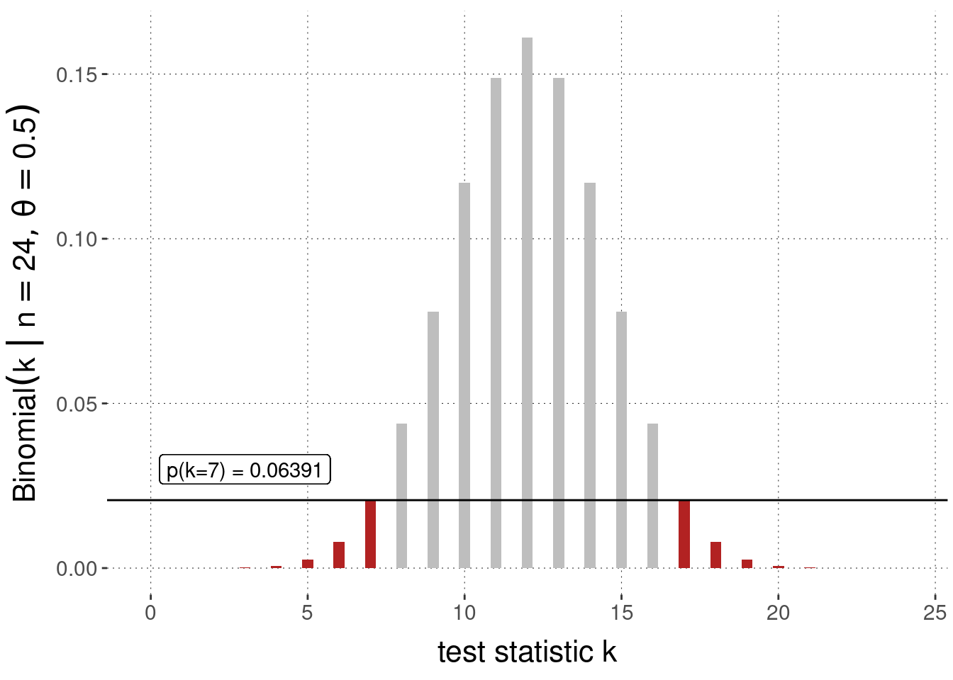
$Sampling distribution (Binomial likelihood function) and two-sided $p$-value for the observation of $k=7$ successes in $N = 24$ coin flips, under the assumption of a null hypothesis $\theta = 0.5$.$

Figure 16.6: Sampling distribution (Binomial likelihood function) and two-sided $p$-value for the observation of $k=7$ successes in $N = 24$ coin flips, under the assumption of a null hypothesis $\theta = 0.5$.

Of course, R also has a built-in function for a Binomial test. We can use it to verify that we get the same result for the $p$-value:

binom.test(
  x = 7,     # observed successes
  n = 24,    # total no. of observations
  p = 0.5    # null hypothesis
)

## 
##  Exact binomial test
## 
## data:  7 and 24
## number of successes = 7, number of trials = 24, p-value = 0.06391
## alternative hypothesis: true probability of success is not equal to 0.5
## 95 percent confidence interval:
##  0.1261521 0.5109478
## sample estimates:
## probability of success 
##              0.2916667

Exercise 16.1: Output of R’s binom.test

Look at the output of the above call to R’s binom.test function. Which pieces of information in that output make sense to you (given your current knowledge) and which do not?

The output given first states what was computed, namely an exact binomial test. You should understand what a binomial test is. The additional adjective exact refers to the fact that we did not use any approximation to get at the shown $p$-value. Next, we see the data repeated and the calculated $p$-value, which we have seen how to calculate by hand. The output then also names the alternative hypothesis, just like the text previously explained, making clear that this is a two-valued $p$-value. Then comes something which you do not yet know about: the notion of a 95% confidence interval will be covered later in this chapter. Finally, the output also gives the maximum likelihood estimate of the theta parameter. Together with the 95% confidence interval, the test result therefore also reports the most common frequentist estimators, point-values (MLE) and interval-valued (95% confidence interval) for the parameter of interest.

Case $\theta > 0.5$. Let’s now look at the case where we want to test whether the coin is biased towards heads $\theta > 0.5$. As explained above, we need a point-valued assumption for the coin bias $\theta$ to set up a frequentist model and retrieve a sampling distribution for the relevant test statistic. We choose $\theta_{0} = 0.5$ as the point-valued null hypothesis, because if we get a high measure of the evidence against the hypothesis $\theta_{0} = 0.5$ (in a comparison against the alternative $\theta < 0.5$), we can discredit the whole interval-based hypothesis $\theta > 0.5$ because any other value of $\theta$ bigger than 0.5 would give at least as high a $p$-value. In other words, we pick the single value for the comparison which is most favorable for the hypothesis $\theta > 0.5$ when compared against $\theta < 0.5$, so as when even that value is discredited, the whole hypothesis $\theta > 0.5$ is discredited.

But even though we use the same null-value of $\theta_0 = 0.5$, the calculation of the $p$-value will be different from the case we looked at previously. It will be one-sided. The reason lies in a change to what we should consider more extreme evidence against this interval-valued null hypothesis, i.e., the interpretation of $\succeq^{H_{0,a}}$. Look at Figure 16.7. As before we see the Bernoulli likelihood function derived from the point-value null hypothesis. The $k$-value observed is $k=7$. Again we need to ask: which values of $k$ would constitute equal or more evidence against the null hypothesis when compared against the alternative hypothesis, which is now $\theta < 0.5$ Unlike in the previous, two-sided case, observing large values of $k$, e.g., larger than 12, even if they are unlikely for the point-valued hypothesis $\theta_0 = 0.5$, does not constitute evidence against the interval-valued hypothesis we are interested in. So therefore, we disregard the contribution of the right-hand side in Figure 16.6 to arrive at a picture like in Figure 16.7.

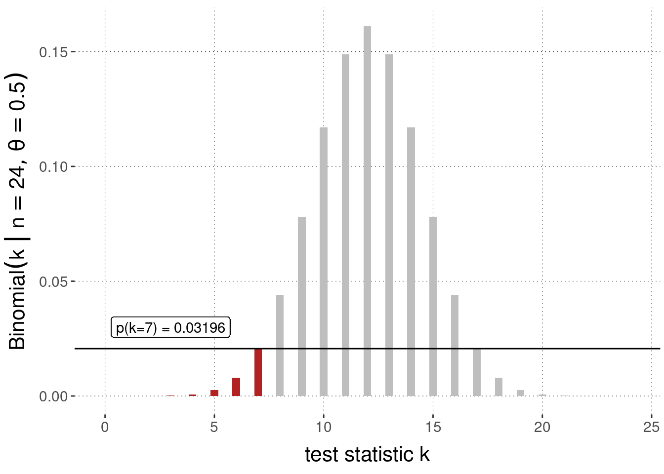
$Sampling distribution (Binomial likelihood function) and one-sided $p$-value for the observation of $k=7$ successes in $N = 24$ coin flips, under the assumption of a null hypothesis $\theta = 0.5$ compared against the alternative hypothesis $\theta < 0$.$

Figure 16.7: Sampling distribution (Binomial likelihood function) and one-sided $p$-value for the observation of $k=7$ successes in $N = 24$ coin flips, under the assumption of a null hypothesis $\theta = 0.5$ compared against the alternative hypothesis $\theta < 0$.

The associated $p$-value with this so-called one-sided test is consequently:

k_obs <- 7
N <- 24
theta_0 <- 0.5
# exact p-value for k = 7 with N = 24 and null hypothesis theta > 0.5
dbinom(0:k_obs, N, theta_0) %>% sum %>% round(5)

## [1] 0.03196

We can double-check against the built-in function binom.test when we ask for a one-sided test:

binom.test(
  x = 7,     # observed successes
  n = 24,    # total no. of observations
  p = 0.5,    # null hypothesis
  alternative = "less" # the alternative to compare against is theta < 0.5
)

## 
##  Exact binomial test
## 
## data:  7 and 24
## number of successes = 7, number of trials = 24, p-value = 0.03196
## alternative hypothesis: true probability of success is less than 0.5
## 95 percent confidence interval:
##  0.0000000 0.4787279
## sample estimates:
## probability of success 
##              0.2916667

16.2.3 Significance & categorical decisions

Fisher’s early writings suggest that he considered $p$-values as quantitative measures of strength of evidence against the null hypothesis. What would need to be done or concluded from such a quantitative measure would need to depend on further careful case-by-base deliberation. In contrast, the Neyman-Pearson approach, as well as the presently practiced hybrid NHST approach use $p$-values to check, in a rigid conventionalized manner, whether a test result is noteworthy in a categorical, not quantitative way. More on the Neyman-Pearson approach in Section 16.4.

Fixing an $\alpha$-level of significance (with common values $\alpha \in \{0.05, 0.01, 0.001\}$), we say that a test result is statistically significant (at level $\alpha$) if the $p$-value of the observed data is lower than the specified $\alpha$. The significance of a test result, as a categorical measure, can then be further interpreted as a trigger for decision making. Commonly, a significant test result is interpreted as the signal to reject the null hypothesis, i.e., to speak and act as if it was false. Importantly, a non-significant test results by some $\alpha$-level is not to be treated as evidence in favor of the null hypothesis.⁷⁹

Exercise 16.2: Significance & errors

If the $p$-value is larger than a prespecified significance threshold $\alpha$ (e.g., $\alpha = 0.05$), we…

…accept $H_0$.
…reject $H_0$ in favor of $H_a$.
…fail to reject $H_0$.

Statement c. is correct.

16.2.4 How (not) to interpret p-values

Though central to much of frequentist statistics, $p$-values are frequently misinterpreted, even by seasoned scientists (Haller and Krauss 2002). To repeat, the $p$-value measures the probability of observing, if the null hypothesis is correct, a value of the test statistic that is (in a specific, contextually specified sense) more extreme than the value of the test statistic that we assign to the observed data. We can therefore treat $p$-values as a measure of evidence against the null hypothesis. And if we want to be even more precise, we interpret this as evidence against the whole assumed data-generating process, a central part of which is the null hypothesis.

The $p$-value is not a statement about the probability of the null hypothesis given the data. So, it is not something like $P(H_0 \mid D)$. The latter is a very appealing notion, but it is one that the frequentist denies herself access to. It can also only be computed based on some consideration of prior plausibility of $H_0$ in relation to some alternative hypothesis. Indeed, to calculate $P(H_0 \mid D)$ is unforgivingly a subjective, Bayesian notion.

Exercise 16.3: $p$-values

Which statement(s) about $p$-values is/are true?

The $p$-value is…

…the probability that the null hypothesis $H_0$ is true.
…the probability that the alternative hypothesis $H_a$ is true.
…the probability, derived from the assumption that $H_0$ is true, of obtaining an outcome for the chosen test statistic that is the exact same as the observed outcome.
…a measure of evidence in favor of $H_0$.
…the probability, derived from the assumption that $H_0$ is true, of obtaining an outcome for the chosen test statistic that is the same as the observed outcome or more extreme evidence for $H_a$.
…a measure of evidence against $H_0$.

Statements e. and f. are correct.

16.2.5 [Excursion] Distribution of $p$-values

A result that might seem surprising at first is that if the null hypothesis is true, the distribution of $p$-values is uniform. This, however, is intuitive on second thought. Mathematically it is a direct consequence of the Probability Integral Transform Theorem.

Theorem 16.1 (Probability Integral Transform) If $X$ is a continuous random variable with cumulative distribution function $F_X$, the random variable $Y = F_X(X)$ is uniformly distributed over the interval $[0;1]$, i.e., $y \sim \text{Uniform}(0,1)$.

Proof. Notice that the cumulative density function of a standard uniform distribution $y \sim \text{Uniform}(0,1)$ is a linear line with intercept 0 and slope 1. It therefore suffices to show that $F_Y(y) = y$. \[ \begin{aligned} F_Y(y) & = P(Y \le y) && [\text{def. of cumulative distribution}] \\ & = P(F_X(X) \le y) && [\text{by construction / assumption}] \\ & = P(X \le F^{-1}_X(y)) && [\text{applying inverse cumulative function}] \\ & = F_X(F^{-1}_X(y)) && [\text{def. of cumulative distribution}] \\ & = y && [\text{inverses cancel out}] \\ \end{aligned} \]

Seeing the uniform distribution of $p$-values (under a true null hypothesis) helps appreciate how the $\alpha$-level of significance is related to long-term error control. If the null hypothesis is true, the probability of a significant test result is exactly the significance level.

References

Haller, Heiko, and Stefan Krauss. 2002. “Misinterpretations of Significance: A Problem Students Share with Their Teachers?” Methods of Psychological Research Online 7 (1): 1–20.

For clarity: the $p$-value is actually a measure of how surprising the data is in light of the whole null-model, which is built around the null hypothesis. As the further ingredients in the null-model are usually considered to be relatively uncontroversial (at least relative to the assumption of the null hypothesis), the $p$-value parlance directly targets the null hypothesis.↩︎
This formulation in terms of a context-dependent, i.e., $H_0$-dependent, ordering is not usual. However, the interpretation is de facto context-dependent in this way, and so it makes sense to highlight this aspect of the use of $p$-values also formally. Notice, however, that we can get rid of the context-dependence by using different test statistics. But this is also not how it is done in practice. Essentially, this definition aims for maximal generality so as to cover all cases of use. Since the class of use cases is fuzzy, the definition needs this flexibility. Alternative mathematical definitions that appear to be simpler just do not capture all the use cases.↩︎
This latter aspect has been particularly important historically. Given more readily available computing power, alternative approaches based on Monte Carlo simulation of $p$-values can also be used.↩︎
It is admittedly a bit of a notational overkill to write this comparison relation as a function of $H_0$ and $H_a$ (the alternative hypothesis). Other definitions of the $p$-value do not. But the comparison is context-dependent, and you deserve to see this clearly. To see it clearly, a certain heaviness of notation is the price to pay.↩︎
Most often, the random variable capturing the sampling distribution is just written as $T$, but it does make sense to stress also notationally that $T$ depends crucially on $H_0$.↩︎
Here, the bracket notation $[ \mathit{Boolean} ]$ is the Iverson bracket, evaluating to 1 if the Boolean expression is true and to 0 otherwise.↩︎
Frequentist hypothesis testing is superficially similar to Popperian falsificationism. It is, however, quite the opposite when looked at more carefully. Popper famously denied that empirical observation could constitute positive evidence in favor of a research hypothesis. Research hypotheses can only be refuted, viz., when their logical consequences are logically incompatible with the observed data. In a Popperian science, what is refuted are research hypotheses; frequentist statistics instead seeks to refute null hypotheses and counts successful refutation of a null hypothesis as evidence in favor of a research hypothesis.↩︎

An Introduction to Data Analysis