10.1 Case study: recall models
As a running example for this chapter, we borrow from Myung (2003) and consider a fictitious data set of recall rates and two models to explain this data.
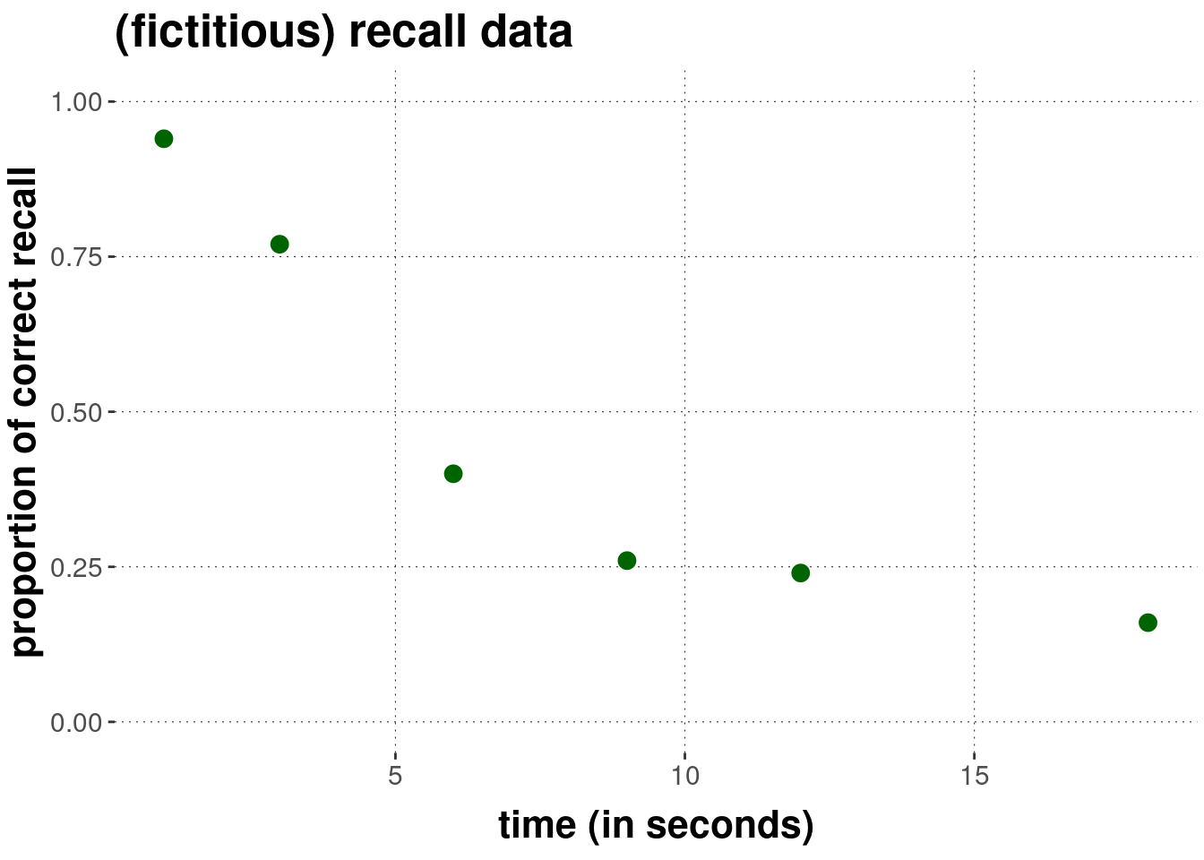
As for the data, for each time point (in seconds) \(t \in \{1, 3, 6, 9, 12, 18\}\), we have 100 (binary) observations of whether a previously memorized item was recalled correctly.
# time after memorization (in seconds)
t <- c(1, 3, 6, 9, 12, 18)
# proportion (out of 100) of correct recall
y <- c(.94, .77, .40, .26, .24, .16)
# number of observed correct recalls (out of 100)
obs <- y * 100
A visual representation of this data set is here:
We are interested in comparing two theoretically different models for this data. Models differ in their assumption about the functional relationship between recall probability and time. The exponential model assumes that the recall probability \(\theta_t\) at time \(t\) is an exponential decay function with parameters \(a\) and \(b\):
\[\theta_t(a, b) = a \exp (-bt), \ \ \ \ \text{where } a,b>0 \]
Taking the binary nature of the data (recalled / not recalled) into account, this results in the following likelihood function for the exponential model:
\[ \begin{aligned} P(k \mid a, b, N , M_{\text{exp}}) & = \text{Binom}(k,N, a \exp (-bt)), \ \ \ \ \text{where } a,b>0 \end{aligned} \]
In contrast, the power model assumes that the relationship is that of a power function:
\[\theta_t(c, d) = ct^{-d}, \ \ \ \ \text{where } c,d>0 \]
The resulting likelihood function for the power model is:
\[ \begin{aligned} P(k \mid c, d, N , M_{\text{pow}}) & = \text{Binom}(k,N, c\ t^{-d}), \ \ \ \ \text{where } c,d>0 \end{aligned} \]
These models therefore make different (parameterized) predictions about the time course of forgetting/recall. Figure 10.1 shows the predictions of each model for \(\theta_t\) for different parameter values:
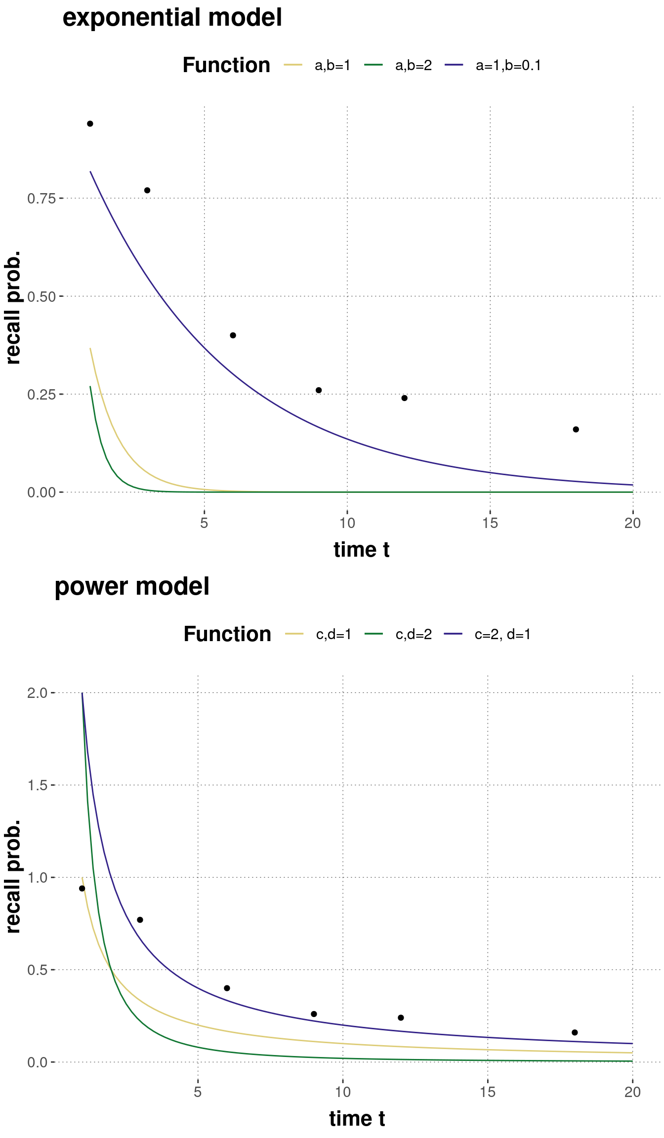
Figure 10.1: Examples of predictions of the exponential and the power model of forgetting for different values of each model’s parameters.
The research question of relevance is: which of these two models is a better model for the observed data? We are going to look at the Akaike information criterion (AIC) first, which only considers the models’ likelihood functions and is therefore a non-Bayesian method. We will see that AIC scores are easy to compute, but give numbers that are hard to interpret or only approximation of quantities that have a clear interpretation. Then we look at a Bayesian method, using Bayes factors, which does take priors over model parameters into account. We will see that Bayes factors are much harder to compute, but do directly calculate quantities that are intuitively interpretable. We will also see that AIC scores only very indirectly take a model’s complexity into account.