16.1 Frequentist statistics: why & how
Bayesian ideas have first been expressed in the 17th century (by Thomas Bayes) and have been given a solid mathematical treatment starting in the 18th century (by French mathematician Pierre-Simon Laplace). A rigorous philosophical underpinning of subjective probability has been given in the early 20th century (by authors like Frank Ramsey or Bruno de Finetti). Still, in the first part of the 20th century, the rise of statistics as a modern, ubiquitous tool for empirical knowledge gain in science took off in a distinctly non-Bayesian direction. Key figures in the early development of statistical ideas (such as Ronald Fisher, Egon Pearson and Jerzy Neyman), were rather opposed to Bayesian ideas. While the precise mechanisms of this historical development are very interesting (from the point of view of history and philosophy of science), suffice it to say here that at least the following two (interrelated) objections are very likely to have contributed a lot to how history unfolded:
- By requiring subjective priors, Bayesian statistical methods have an air of vagueness and non-rigidity.
- Bayesian inference is very demanding (mathematically and computationally).71
As an alternative to Bayesian approaches, the dominant method of statistical inference of the 20th century is frequentist statistics. As a matter of strong philosophical conviction, frequentist statistics makes do entirely without subjective probability: no priors on parameters, no priors on models, no researcher beliefs whatsoever. A crude (and certainly simplified) explanation of why frequentist approaches eschew subjective beliefs is this. Extreme frequentism denies that a probability distribution over a latent parameter like \(\theta\) is meaningful. Whatever we choose, the choice cannot be justified or defended in a scientifically rigorous manner. The only statements about probabilities that are conceptually sound, according to a fundamentalist frequentist interpretation, are those that derive from intuitions about limiting frequencies when (hypothetically) performing a random process (like throwing a dice or drawing a ball from an urn) repeatedly. Bluntly put, there is no “(thought) experiment” which can be repeated so that its objective results, on average, align with whatever subjective prior beliefs the Bayesian analysis needs.
Of course, the objections to the use of priors could be less fundamentalist. Researchers who have no metaphysical troubles with subjective priors in principle might reject the use of priors in data analysis because they feel that the necessity to specify priors is a burden or a spurious degree of freedom in empirical science. Thus, priors should be avoided to stay as objective, procedurally systematic, and streamlined as possible.
So, after having seen Bayesian inference in action extensively, you may wonder: how -on earth- is inference and hypothesis testing even possible without (subjective) priors, even if assumed to be non-informative? - Frequentist statistics has devised very clever means of working around subjective probability. Frequentists do accept probabilities, of course. But only of the objective kind: in the form of a likelihood function which can be justified by appeal to repeated executions and limiting frequencies of events. In a (simplified) nutshell, you may think of frequentism as squeezing everything (inference, estimation, testing, model comparison) out of suitably constructed likelihood functions, which are constructed around point-valued assumptions about any remaining model parameters.
Central to frequentist statistics is the notion of a \(p\)-value, which plays a central role in hypothesis testing. Let’s consider an example. The goal is to get a first idea of how frequentist methods can work without subjective probability. More detail will be presented in the following sections. Say, we are interested in the question of whether a given coin is fair, so: \(\theta_c = 0.5\). This assumption \(\theta_{c} = 0.5\) is our null hypothesis \(H_{0}\).72 We refuse to express beliefs about the likely value of \(\theta_c\), both prior and posterior. But we are allowed to engage in hypothetical mind games. So, let’s assume for the sake of argument that the coin is fair. So, we assume the null hypothesis to be true for the sake of argument. That’s not a belief; it’s a thought experiment: nothing wrong with that. We build a frequentist model around this point-valued assumption, and call it a null-model. The null-model assumes that \(\theta_{c} = 0.5\) but also uses the obvious likelihood function, \(\text{Binomial}(k, N, \theta_c = 0.5)\), stating how likely it would be to observe \(k\) heads in \(N\) tosses, for fixed \(\theta_c = 0.5\). These likelihoods are not subjective, but grounded in limiting frequencies of events. Now, we also bring into the picture some actual data. Unsurprisingly: \(k=7\), \(N=24\). We can now construct a measure of how surprising this data observation would be on the purely instrumental assumption that the null-model is true. In more Bayesian words, we are interested in measuring the perplexity of an agent whose belief is captured by the null-model (so an agent who genuinely and inflexibly believes that the coin is fair), when that agent observes \(k=7\) and \(N=24\). If the agent’s perplexity is extremely high, i.e., if the null-model would not have predicted the data at hand to a high enough degree, we take this as evidence against the null-model. Since the main contestable assumption in the construction of the null-model is the null hypothesis itself, we treat this as evidence against the null hypothesis, and so are able to draw conclusions about a point-valued hypothesis of interest, crucially, without any recourse to subjective probability. The quantified notion of evidence against a null-model is the \(p\)-value, famously introduced by Ronald Fisher, which we will discuss in the next section 16.2.
Historically, there have been different schools of thought in frequentist statistics, all of which relate in some way or other to a quantified notion of evidence against a null-model, but that differ substantially in other ways. The three main approaches, shown in Figure 16.1, are Fisher’s approach, the Neyman-Pearson approach and the hybrid approach, often referred to simply as NHST (= null hypothesis significance testing), which is the standard practice today. In simplified terms, the main difference is that Fisher’s approach is belief-oriented, while the Neyman-Pearson approach is action-oriented. Fisher’s approach calculates \(p\)-values as measures of evidence against a model, but does not necessarily prescribe what to do with this quantitative measure. The approach championed by Neyman-Pearson calculates a \(p\)-value and also fixes categorical decision rules relating to whether to accept or reject the null-model (or an alternative model, which is also explicitly featured in the Neyman-Pearson approach). The main rationale for the Neyman-Pearson approach is to to have a tight upper bound on certain types of statistical error. Section 16.4 deals with the Neyman-Pearson approach in more detail, where we also introduce the notion of statistical significance.
While both Fisher’s approach and the Neyman-Pearson approach are intrinsically sound, in actual practice we often see a rather inconsistent mix of ideas and practices. That’s why Figure 16.1 characterizes the modern NHST approach more in terms of how we actually find it applied in practice (and, unfortunately, also taught) rather than how it should be.
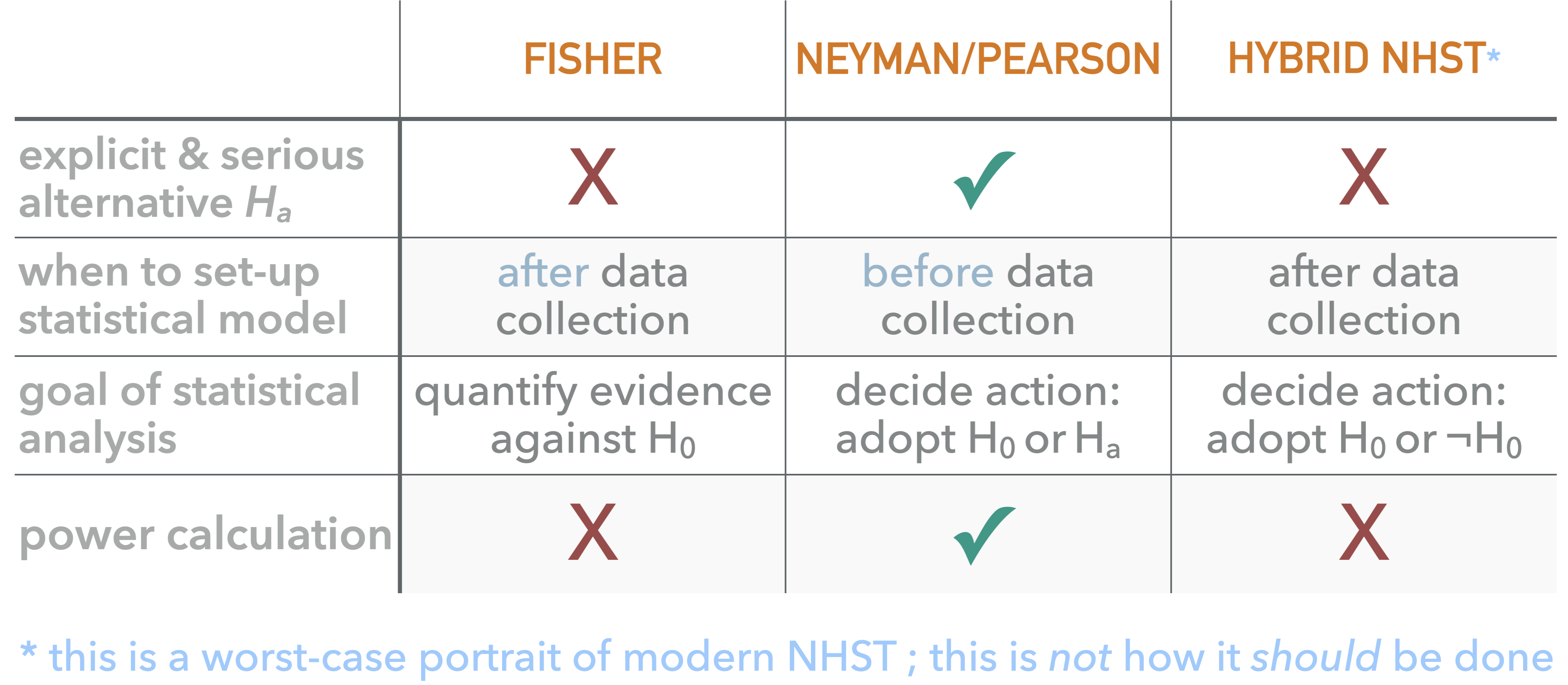
Figure 16.1: The three most prominent flavors of frequentist statistics.
References
Notice also that Bayesian computation is a very recent field. The MCMC algorithm was only invented in the middle of the 20th century. Before close to the turn of the 21st century, researchers lacked wide-spread access to computers powerful enough to run algorithms that approximate Bayesian inference for complex models.↩︎
The term “null hypothesis” does not want to imply that the hypothesis is that some value of interest is equal to zero (although in practice that is frequently the case). The term rather implicates that this hypothesis is put out there in order to be possibly refuted, i.e., nullified, by the data (Gigerenzer 2004).↩︎