expected_value <- 1*(1/6) + 2*(1/6) + 3*(1/6) + 4*(1/6) + 5*(1/6) + 6*(1/6)
variance <- 1^2*(1/6) + 2^2*(1/6) + 3^2*(1/6) + 4^2*(1/6) + 5^2*(1/6) + 6^2*(1/6) - expected_value^2

print(expected_value)
## [1] 3.5variance## [1] 2.916667So far, we have defined a probability distribution as a function that assigns a probability to each subset of the space \(\Omega\) of elementary outcomes. We saw that rational beliefs should conform to certain axioms, reflecting a “logic of rational beliefs”. But in data analysis, we are often interested in a space of numeric outcomes. You probably know stuff like the “normal distribution” which is a distribution that assigns a probability to each real number. In keeping with our previous definition of probability as targeting a measurable set \(\Omega\), we introduce what we could sloppily call “probability distributions over numbers” using the concept of random variables. Caveat: random variables are very useful concepts and offer highly versatile notation, but both concept and notation can be elusive in the beginning.
Formally, a random variable is a function \(X \ \colon \ \Omega \rightarrow \mathbb{R}\) that assigns to each elementary outcome a numerical value. It is reasonable to think of this number as a summary statistic: a number that captures one aspect of relevance of what is actually a much more complex chunk of reality.
Traditionally, random variables are represented by capital letters, like \(X\). The numeric values they take on are written as small letters, like \(x\).
We write \(P(X = x)\) as a shorthand for the probability \(P(\left \{ \omega \in \Omega \mid X(\omega) = x \right \})\), that an event \(\omega\) occurs which is mapped onto \(x\) by the random variable \(X\). For example, if our coin is fair, then \(P(X_{\text{two flips}} = x) = 0.5\) for \(x=1\) and \(0.25\) for \(x \in \{0,2\}\). Similarly, we can also write \(P(X \le x)\) for the probability of observing any event that \(X\) maps to a number not bigger than \(x\).
If the range of \(X\) is countable (not necessarily finite), we say that \(X\) is discrete. For ease of exposition, we may say that if the range of \(X\) is an interval of real numbers, \(X\) is called continuous.
For a discrete random variable \(X\), the cumulative distribution function \(F_X\) associated with \(X\) is defined as: \[ F_X(x) = P(X \le x) = \sum_{x' \in \left \{ x'' \in \text{range}(X) \mid x'' \le x \right \}} P(X = x') \] The probability mass function \(f_x\) associated with \(X\) is defined as: \[ f_X(x) = P(X = x) \]
Example. Suppose we flip a coin with a bias of \(\theta\) towards heads \(n\) times. What is the probability that we will see heads \(k\) times? If we map the outcome of heads to 1 and tails to 0, this probability is given by the Binomial distribution, as follows: \[ \text{Binom}(K = k ; n, \theta) = \binom{n}{k} \, \theta^{k} \, (1-\theta)^{n-k} \] Here \(\binom{n}{k} = \frac{n!}{k!(n-k)!}\) is the binomial coefficient, which gives the number of possibilities of drawing an unordered subset with \(k\) elements from a set with a total of \(n\) elements. Figure 7.3 gives examples of the Binomial distribution, concretely its probability mass functions, for two values of the coin’s bias, \(\theta = 0.25\) or \(\theta = 0.5\), when flipping the coin \(n=24\) times. Figure 7.4 gives the corresponding cumulative distributions.
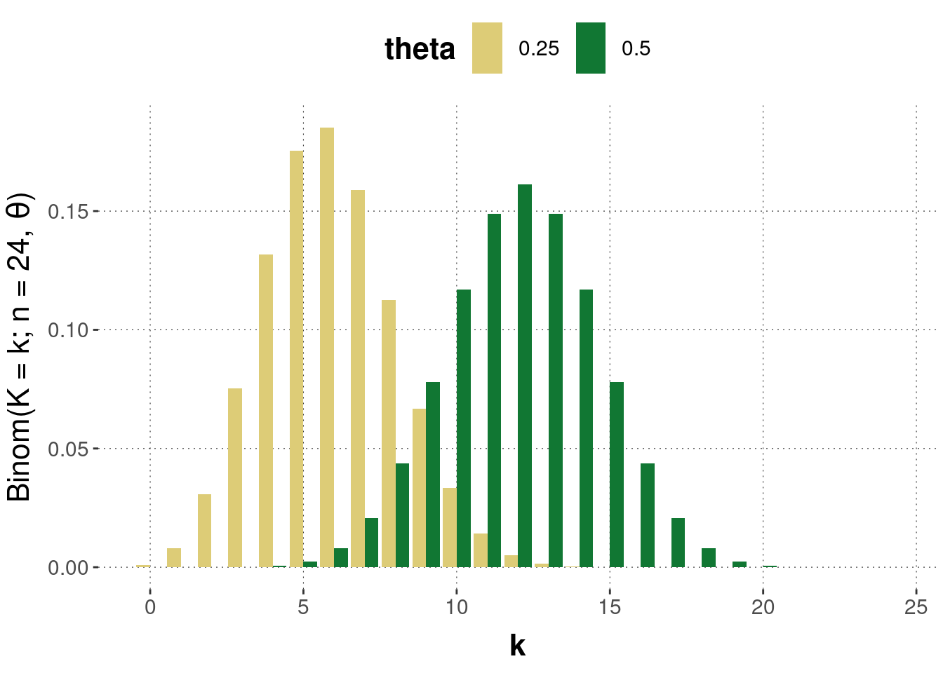
Figure 7.3: Examples of the Binomial distribution. The \(y\)-axis gives the probability of seeing \(k\) heads when flipping a coin \(n=24\) times with a bias of either \(\theta = 0.25\) or \(\theta = 0.5\).
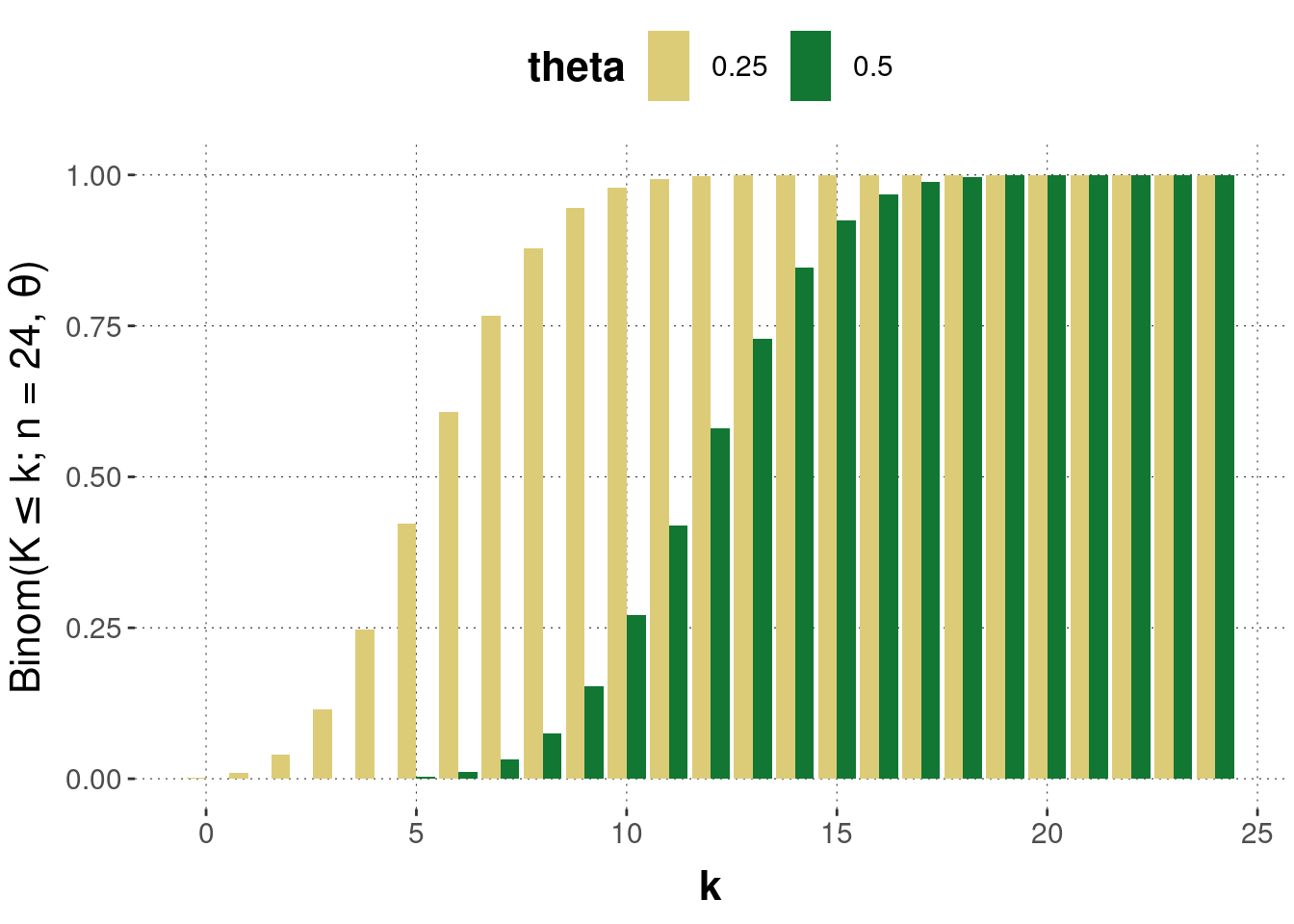
Figure 7.4: Examples of the cumulative distribution of the Binomial distribution. The \(y\)-axis gives the probability of seeing \(k\) or fewer outcomes of heads when flipping a coin \(n=24\) times with a bias of either \(\theta = 0.25\) or \(\theta = 0.5\).
For a continuous random variable \(X\), the probability \(P(X = x)\) will usually be zero: it is virtually impossible that we will see precisely the value \(x\) realized in a random event that can realize uncountably many numerical values of \(X\). However, \(P(X \le x)\) does usually take non-zero values and so we define the cumulative distribution function \(F_X\) associated with \(X\) as: \[ F_X(x) = P(X \le x) \] Instead of a probability mass function, we derive a probability density function from the cumulative function as: \[ f_X(x) = F'(x) \] A probability density function can take values greater than one, unlike a probability mass function.
Example. The Gaussian (Normal) distribution characterizes many natural distributions of measurements which are symmetrically spread around a central tendency. It is defined as: \[ \mathcal{N}(X = x ; \mu, \sigma) = \frac{1}{\sqrt{2 \sigma^2 \pi}} \exp \left ( - \frac{(x-\mu)^2}{2 \sigma^2} \right) \] where parameter \(\mu\) is the mean, the central tendency, and parameter \(\sigma\) is the standard deviation. Figure 7.5 gives examples of the probability density function of two normal distributions. Figure 7.6 gives the corresponding cumulative distribution functions.
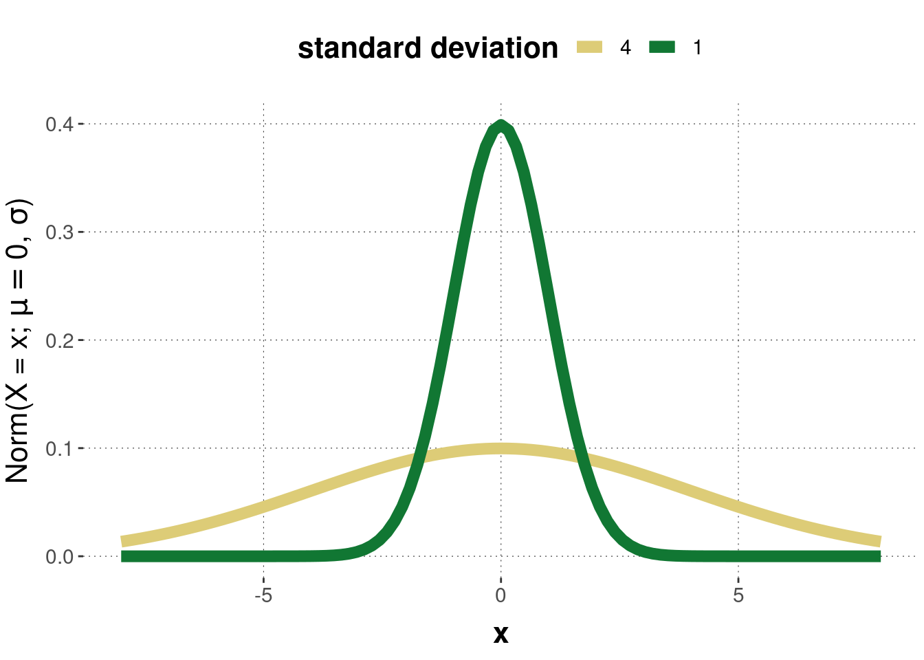
Figure 7.5: Examples of the Normal distribution. In both cases \(\mu = 0\), once with \(\sigma = 1\) and once with \(\sigma = 4\).
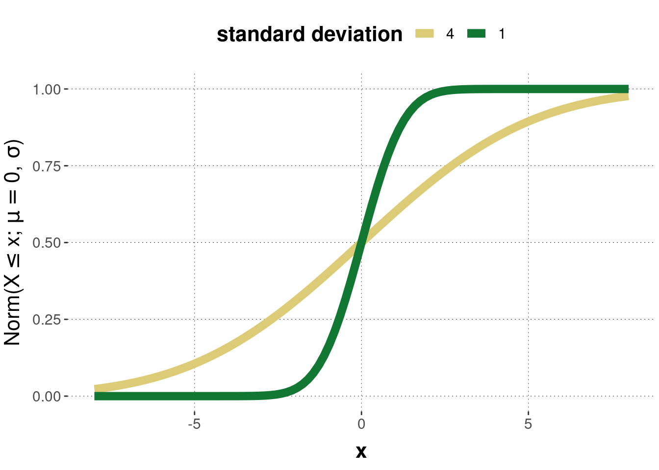
Figure 7.6: Examples of the cumulative normal distribution corresponding to the previous probability density functions.
The expected value of a random variable \(X\) is a measure of central tendency. It tells us, like the name suggests, which average value of \(X\) we can expect when repeatedly sampling from \(X\). If \(X\) is discrete, the expected value is: \[ \mathbb{E}_X = \sum_{x} x \times f_X(x) \] If \(X\) is continuous, it is: \[ \mathbb{E}_X = \int x \times f_X(x) \ \text{d}x \] The expected value is also frequently called the mean.
The variance of a random variable \(X\) is a measure of how much likely values of \(X\) are spread or clustered around the expected value. If \(X\) is discrete, the variance is: \[ \text{Var}(X) = \sum_x (\mathbb{E}_X - x)^2 \times f_X(x) = \mathbb{E}_{X^2} -\mathbb{E}_X^2 \] If \(X\) is continuous, it is: \[ \text{Var}(X) = \int (\mathbb{E}_X - x)^2 \times f_X(x) \ \text{d}x = \mathbb{E}_{X^2} -\mathbb{E}_X^2 \]
Example. If we flip a coin with bias \(\theta = 0.25\) a total of \(n=24\) times, we expect on average to see \(n \times\theta = 24 \times 0.25 = 6\) outcomes showing heads.42 The variance of a binomially distributed variable is \(n \times\theta \times(1-\theta) = 24 \times 0.25 \times 0.75 = \frac{24 \times 3}{16} = \frac{18}{4} = 4.5\).
The expected value of a normal distribution is just its mean \(\mu\) and its variance is \(\sigma^2\).
Exercise 7.5
expected_value <- 1*(1/6) + 2*(1/6) + 3*(1/6) + 4*(1/6) + 5*(1/6) + 6*(1/6)
variance <- 1^2*(1/6) + 2^2*(1/6) + 3^2*(1/6) + 4^2*(1/6) + 5^2*(1/6) + 6^2*(1/6) - expected_value^2
print(expected_value)## [1] 3.5variance## [1] 2.916667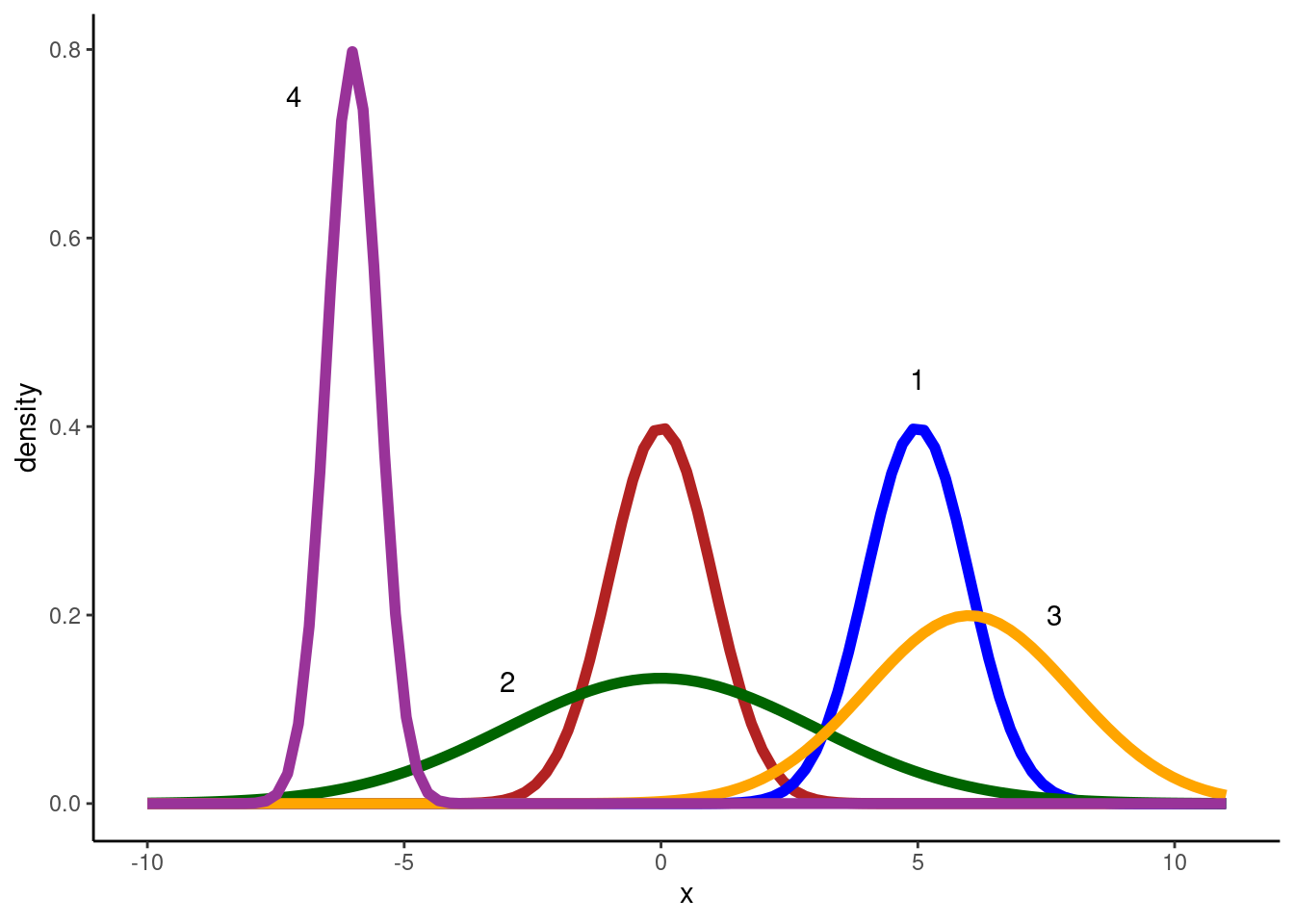
Distribution 1 (\(\mu\) = 5, \(\sigma\) = 1): larger mean, same standard deviation
Distribution 2 (\(\mu\) = 0, \(\sigma\) = 3): same mean, larger standard deviation
Distribution 3 (\(\mu\) = 6, \(\sigma\) = 2): larger mean, larger standard deviation
Distribution 4 (\(\mu\) = -6, \(\sigma\) = 0.5): smaller mean, smaller standard deviation
Composite random variables are random variables generated by mathematical operations conjoining other random variables. For example, if \(X\) and \(Y\) are random variables, then we can define a new derived random variable \(Z\) using notation like:
\[Z = X + Y\]
This notation looks innocuous but is conceptually tricky yet ultimately very powerful. On the face of it, we are doing as if we are using + to add two functions. But a sampling-based perspective makes this quite intuitive. We can think of \(X\) and \(Y\) as large samples, representing the probability distributions in question. Then we build a sample by just adding elements in \(X\) and \(Y\). (If samples are of different size, just add a random element of \(Y\) to each \(X\).)
Consider the following concrete example. \(X\) is the probability distribution of rolling a fair dice with six sides. \(Y\) is the probability distribution of flipping a biased coin that lands heads (represented as number 1) with probability 0.75. The derived probability distribution \(Z = X + Y\) can be approximately represented by samples derived as follows:
n_samples <- 1e6
# `n_samples` rolls of a fair dice
samples_x <- sample(
  1:6,
  size = n_samples,
  replace = T
)

# `n_samples` flips of a biased coin
samples_y <- sample(
  c(0, 1),
  prob = c(0.25, 0.75),
  size = n_samples,
  replace = T
)

samples_z <- samples_x + samples_y

tibble(outcome = samples_z) %>%
  dplyr::count(outcome) %>%
  mutate(n = n / sum(n)) %>%
  ggplot(aes(x = outcome, y = n)) +
  geom_col() +
  labs(y = "proportion")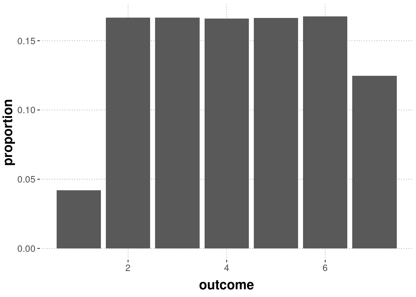
This is not immediately obvious from our definition, but it is intuitive and you can derive it.↩︎