5 * (659 - 34)## [1] 3125R is an interpreted language. This means that you do not have to compile it. You can just evaluate it line by line, in a so-called session. The session stores the current values of all variables. Usually, code is stored in a script, so one does not have to retype it when starting a new session. 2
Try this out by either typing r to open an R session in a terminal or load RStudio.3 You can immediately calculate stuff:
6 * 7## [1] 42Exercise 2.1 Use R to calculate 5 times the result of 659 minus 34.
5 * (659 - 34)## [1] 3125R has many built-in functions. The most common situation is that the function is called by its name using prefix notation, followed by round brackets that enclose the function’s arguments (separated by commas if there are multiple arguments). For example, the function round takes a number and, by default, returns the closest integer:
# the function `round` takes a number as an argument and
# returns the closest integer (default)
round(0.6)
## [1] 1Actually, round allows several arguments. It takes as input the number x to be rounded and another integer number digits which gives the number of digits after the comma to which x should be rounded. We can then specify these arguments in a function call of round by providing the named arguments.
# rounds the number `x` to the number `digits` of digits
round(x = 0.138, digits = 2)
## [1] 0.14If all of the parsed arguments are named, then their order does not matter. But all non-named arguments have to be presented in the positions expected by the function after subtracting the named arguments from the ordered list of arguments (to find out the right order one should use help, as explained below in 2.1.6). Here are examples for illustration:
round(x = 0.138, digits = 2)  # works as intended
round(digits = 2, x = 0.138)  # works as intended
round(0.138, digits = 2)      # works as intended
round(0.138, 2)               # works as intended
round(x = 0.138, 2)           # works as intended
round(digits = 2, 0.138)      # works as intended
round(2, x = 0.138)           # works as intended
round(2, 0.138)               # does not work as intended (returns 2)
Functions can have default values for some or for all of their arguments. In the case of round, the default is digits = 0. There is obviously no default for x in the function round.
round(x = 6.138) # returns 6## [1] 6Some functions can take an arbitrary number of arguments. The function sum, which sums up numbers is a point in case.
# adds all of its arguments together
sum(1, 2, 3)
## [1] 6Selected functions can also be expressed as operators in infix notation. This applies to frequently recurring operations, such as mathematical operations or logical comparisons.
# both of these calls sum 1, 2, and 3 together
sum(1, 2, 3)   # prefix notation
1 + 2 + 3      # infix notation
An expression like 3 + 5 is internally processed as the function `+`(3, 5) which is equivalent to sum(3, 5).
Section 2.3 will list some of the most important built-in functions. It will also explain how to define your own functions.
You can assign values to variables using three assignment operators: ->, <- and =, like so:
x <- 6       # assigns 6 to variable x
7 -> y       # assigns 7 to variable y
z = 3        # assigns 3 to variable z
x * y / z    # returns 6 * 7 / 3 = 14
## [1] 14Use of = is discouraged.4
It is good practice to use a consistent naming scheme for variables. This book uses snake_case_variable_names and tends towards using long_and_excessively_informative_names for important variables, and short variable names, like i, j or x, for local variables, indices etc.
Exercise 2.2
Create two variables, a and b, and assign the values 103 and 14 to them, respectively. Next, divide variable a by variable b and produce an output with three digits after the comma.
a <- 103
b <- 14
round(x = a / b, digits = 3)
## [1] 7.357It is good practice to document code with short but informative comments. Comments in R are demarcated with #.
x <- 4711 # a nice number from CologneSince everything on a line after an occurrence of # is treated as a comment, it is possible to break long function calls across several lines, and to add comments to each line:
round(            # call the function `round`
  x = 0.138,      # number to be rounded
  digits = 2      # number of after-comma digits to round to
)
In RStudio, you can use Command+Shift+C (on Mac) and Ctrl+Shift+C (on Windows/Linux) to comment or uncomment code, and you can use comments to structure your scripts. Any comment followed by ---- is treated as a (foldable) section in RStudio.
# SECTION: variable assignments ----
x <- 6
y <- 7
# SECTION: some calculations ----
x * y
Exercise 2.3
Provide extensive comments to all operations in the solution code of the previous exercise.
a <- 103   # assign value 103 to variable `a`
b <- 14    # assign value 14 to variable `b`
round(     # produce a rounded number
  x = a / b,   # number to be rounded is a/b
  digits = 3   # show three digits after the comma
)
## [1] 7.357Strictly speaking, all entities in R are objects but that is not always apparent or important for everyday practical purposes (see the manual for more information). R supports an object-oriented programming style, but we will not make (explicit) use of this functionality. In fact, this book heavily uses and encourages a functional programming style (see Section 2.4).
However, some functions (e.g., optimizers or fitting functions for statistical models) return objects, and we will use this output in various ways. For example, if we run some model on a data set the output is an object. Here, for example, we run a regression model, that will be discussed later on in the book, on a dataset called cars.
# you do not need to understand this code
model_fit = lm(formula = speed~dist, data = cars)
# just notice that the function `lm` returns an object
is.object(model_fit)
## [1] TRUE# printing an object on the screen usually gives you summary information
print(model_fit)##
## Call:
## lm(formula = speed ~ dist, data = cars)
##
## Coefficients:
## (Intercept) dist
## 8.2839 0.1656Much of R’s charm unfolds through the use of packages. CRAN has the official package repository. To install a new package from a CRAN mirror use the install.packages function. For example, to install the package remotes, you would use:
install.packages("remotes")Once installed, you need to load your desired packages for each fresh session, using a command like the following:5
library(remotes)Once loaded, all functions, data, etc. that ship with a package are available without additional reference to the package name. If you want to be careful or courteous to an admirer of your code, you can reference a function from a package also by explicitly referring to that package. For example, the following code calls the function install_github from the package remotes explicitly.6
remotes::install_github("SOME-URL")Indeed, the install_github function allows you to install bleeding-edge packages from GitHub. You can install all packages relevant for this book using the following code (after installing the remotes package):
remotes::install_github("michael-franke/aida-package")After this installation, you can load all packages for this book simply by using:
library(aida)In RStudio, there is a special tab in the pane with information on “files”, “plots” etc. to show all installed packages. This also shows which packages are currently loaded.
If you encounter a function like lm that you do not know about, you can access its documentation with the help function or just typing ?lm. For example, the following call summons the documentation for lm, the first parts of which are shown in Figure 2.2.
help(lm)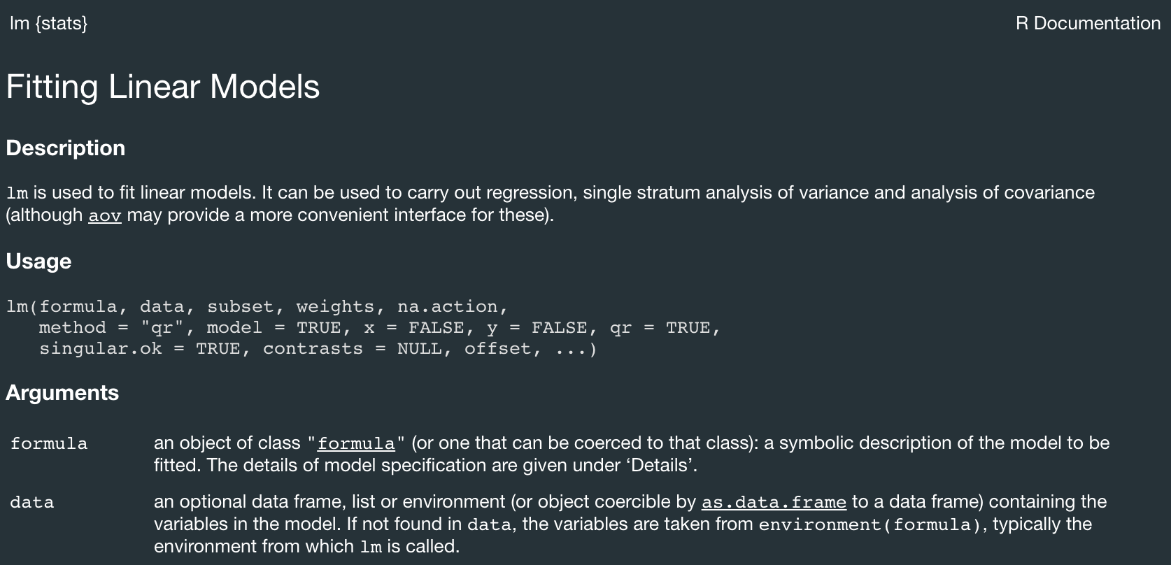
Figure 2.2: Excerpt from the documentation of the lm function.
If you are looking for help on a more general topic, use the function help.search. It takes a regular expression as input and outputs a list of occurrences in the available documentation. A useful shortcut for help.search is just to type ?? followed by the (unquoted) string to search for. For example, calling either of the following lines might produce a display like in Figure 2.3.
# two equivalent ways for obtaining help on search term 'linear'
help.search("linear")
??linear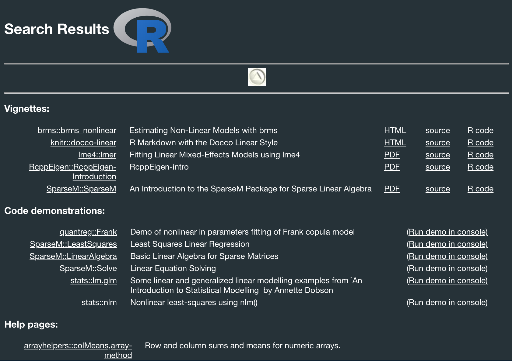
Figure 2.3: Result of calling help.search for the term ‘linear’.
The top entries in Figure 2.3 are vignettes. These are compact manuals or tutorials on particular topics or functions, and they are directly available in R. If you want to browse through the vignettes available on your machine (which depend on which packages you have installed), go ahead with:
browseVignettes()Exercise 2.4
Look up the help page for the command round. As you know about this function already, focus on getting a feeling for how the help text is structured and the most important bits of information are conveyed. Try to understand what the other functions covered in this entry do and when which one would be most useful.
Line-by-line execution of code is useful for quick development and debugging. Make sure to learn about keyboard shortcuts to execute single lines or chunks of code in your favorite editor, e.g., check the RStudio Cheat Sheet for information on its keyboard shortcuts.↩︎
You might need to add R to the PATH variables of your operating system to let the terminal know where R was installed (e.g. C:\Program Files\R\R-4.0.3\bin\x64). Also, when starting a session in a terminal, you can exit a running R session by typing quit() or q().↩︎
You can produce <- in RStudio with Option-- (on Mac) and Alt-- (on Windows/Linux). For other useful keyboard shortcuts, see here.↩︎
You need to make sure that all packages you need for a session are loaded, so you would need to supply several commands like library(PCKG_NAME) for all required packages.↩︎
Calling functions in this explicit way also dispenses the need to load the package first (though you need to have installed it before), and it might help with naming conflicts when different packages define identically named functions.↩︎