The 0/1 coding scheme above works fine for a single categorical predictor value with two levels.
It is possible to use linear regression also for categorical predictors with more than two levels.
Only, in that case, there are quite a few more reasonable contrast coding schemes, i.e., ways to choose numbers to encode the levels of the predictor.
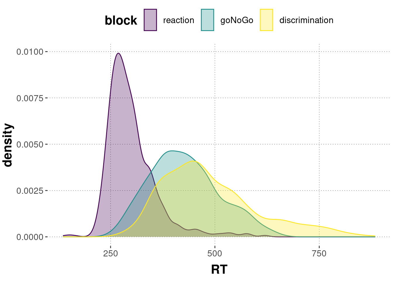
The mental chronometry data has a single categorical predictor, called block, with three levels, called “reaction”, “goNoGo” and “discrimination”.
We are interested in regressing reaction times, stored in variable RT, against block.
Our main question of interest is whether these inequalities are supported by the data:
\[
\text{RT in 'reaction'} <
\text{RT in 'goNoGo'} <
\text{RT in 'discrimination'}
\]
So we are interested in the \(\delta\)s, so to speak, between ‘reaction’ and ‘goNoGo’ and between ‘discrimination’ and ‘goNoGo’.
Let’s consider only the data relevant for our current purposes:
# select the relevant columnsdata_MC_excerpt <- aida::data_MC_cleaned %>%select(RT, block)# show the first couple of linesdata_MC_excerpt %>%head(5)
And here is a plot of the distribution of measurements in each block:
To fit this model with brms, we need a simple function call with the formula RT ~ block that precisely describes what we are interested in, namely explaining reaction times as a function of the experimental condition:
Notice that there is an intercept term, as before.
This corresponds to the mean reaction time of the reference level, which is again set based on alphanumeric ordering, so corresponding to “discrimination”.
There are two slope coefficients, one for the difference between the reference level and “goNoGo” and another for the difference between the reference level and the “reaction” condition.
These intercepts are estimated to be credibly negative, suggesting that the “discrimination” condition indeed had the highest mean reaction times.
This answers one half of the comparisons we are interested in:
\[
\text{RT in 'reaction'} <
\text{RT in 'goNoGo'} <
\text{RT in 'discrimination'}
\]
Unfortunately, it is not directly possible to read off information about the second comparison we care about, namely the comparison between “reaction” and “goNoGo”.
And here is where we see the point of contrast coding pop up for the first time.
We would like to encode predictor levels ideally in such a way that we can read off (test) the hypotheses we care about directly.
In other words, if possible, we would like to have parameters in our model in the form of slope coefficients, which directly encode the \(\delta\)s, so to speak, that we want to test.65
In the case at hand, all we need to do is change the reference level.
If the reference level is the “middle category” (as per our ordered hypothesis), the two slopes will express the contrasts we care about.
To change the reference level, we only need to make block a factor and order its levels manually, like so:
Now the “Intercept” corresponds to the new reference level “goNoGo”.
And the two slope coefficients give the differences to the other two levels.
Which numeric encoding leads to this result?
In formulaic terms, we have three coefficients \(\beta_0, \dots, \beta_2\).
The predicted mean value for observation \(i\) is \(\xi_i = \beta_0 + \beta_1 x_{i1} + \beta_2 x_{i2}\).
We assign numeric value \(1\) for predictor \(x_1\) when the observation is from the “reaction” block.
We assign numeric value \(1\) for predictor \(x_2\) when the observation is from the “discrimination” block.
Schematically, what we now have is:
As we may have expected, the 95% inter-quantile range for both slope coefficients (which, given the amount of data we have, is almost surely almost identical to the 95% HDI) does not include 0 by a very wide margin.
We could therefore conclude that, based on a Bayesian approach to hypothesis testing in terms of posterior estimation, the reaction times of conditions are credibly different.
The coding of levels in terms of a reference level is called treatment coding, or also dummy coding.
The video included at the beginning of this chapter discusses further contrast coding schemes, and also shows in more detail how a coding scheme translates into “directly testable” hypotheses.
Exercise 14.2
Suppose that there are three groups, A, B, and C as levels of your predictor. You want the regression intercept to be the mean of group A. You want the first slope to be the difference between the means of group B and group A. And, you want the second slope to be the difference between the mean of C and B. How do you numerically encode these contrasts in terms of numeric predictor values?
Schematically, like this:
## # A tibble: 3 × 4
##   group   x_0   x_1   x_2
##   <chr> <dbl> <dbl> <dbl>
## 1 A         1     0     0
## 2 B         1     1     0
## 3 C         1     1     1
As group A is a reference category, \(\beta_0\) expresses the mean reaction time of group A. The mean reaction time of group B is \(\beta_0 + \beta_1\), so we need \((x_{i1} =1 , x_{i2} = 0)\) for any \(i\) which is of group B. In the text above, the mean reaction time of group C is given by \(\beta_0 + \beta_2\). However, the value we need now is given by \(\beta_0 + \beta_1 + \beta_2\), so \((x_{i1} =1 , x_{i2} = 1)\).
To be precise, it is possible to also test derived random variables from the posterior samples. So, it is not necessary to encode the contrasts of interests directly. But, most often, in Bayesian analyses it will make sense to put priors on exactly these \(\delta\)s (e.g., skeptical priors biased against a hypothesis to be tested) and for that purpose, it is (almost) practically necessary to have the relevant contrasts expressed as slope coefficients in the model.↩︎