Cheat sheet: common things to do with BRMS

Bayesian regression: theory & practice

Author

Michael Franke

This document provides a cursory run-down of common operations and manipulations for working with the brms package.

Preamble

Here is code to load (and if necessary, install) required packages, and to set some global options (for plotting and efficient fitting of Bayesian models).

Toggle code
# install packages from CRAN (unless installed)
pckgs_needed <- c(
  "tidyverse",
  "brms",
  "rstan",
  "rstanarm",
  "remotes",
  "tidybayes",
  "bridgesampling",
  "shinystan",
  "mgcv"
)
pckgs_installed <- installed.packages()[,"Package"]
pckgs_2_install <- pckgs_needed[!(pckgs_needed %in% pckgs_installed)]
if(length(pckgs_2_install)) {
  install.packages(pckgs_2_install)
} 

# install additional packages from GitHub (unless installed)
if (! "aida" %in% pckgs_installed) {
  remotes::install_github("michael-franke/aida-package")
}
if (! "faintr" %in% pckgs_installed) {
  remotes::install_github("michael-franke/faintr")
}
if (! "cspplot" %in% pckgs_installed) {
  remotes::install_github("CogSciPrag/cspplot")
}

# load the required packages
x <- lapply(pckgs_needed, library, character.only = TRUE)
library(aida)
library(faintr)
library(cspplot)

# these options help Stan run faster
options(mc.cores = parallel::detectCores())

# use the CSP-theme for plotting
theme_set(theme_csp())

# global color scheme from CSP
project_colors = cspplot::list_colors() |> pull(hex)
# names(project_colors) <- cspplot::list_colors() |> pull(name)

# setting theme colors globally
scale_colour_discrete <- function(...) {
  scale_colour_manual(..., values = project_colors)
}
scale_fill_discrete <- function(...) {
   scale_fill_manual(..., values = project_colors)
}

Running a regression model

As a running example, we fit a multi-level model.

Toggle code
data_MC <- aida::data_MC_preprocessed |> 
      mutate(condition = factor(as.character(block), 
                                levels = c("goNoGo", "reaction", "discrimination")))

fit_MC <- 
  brms::brm(
    # "brmsformula" object specifies the model to fit
    formula = RT ~ condition + (1 + condition + shape | submission_id),
    # data to fit model to
    data = data_MC,
    # "iter" is the number of iterations
    iter = 4000,
    # control parameters for MCMC
    control = list(adapt_delta = 0.9)
  )

Updating a model

Using stats::update(), refit a model based on an existing model fit, keeping everything as is, except for what is explicitly set:

Toggle code
# take existing fit, refit on smaller data set, just take 100 samples (all else equal)
fit_first_five <- 
  stats::update(
    object = fit_MC,
    iter = 100,
    # use first five participants only
    newdata = data_MC |> filter(submission_id >= 8550)
  )

Formula syntax

The basic form of a brms formula is: response ~ pterms + (gterms | group)

Multi-level modeling

  • (gterms || group) : suppress correlation between gterms
  • (gterms | g1 + g2) : syntactic sugar for (gterms | g1) + (gterms | g2)
  • (gterms | g1 : g2) : all combinations of g1 and g2 (Cartesian product)
  • (gterms | g1 / g2) : nesting g2 within g1; equals (gterms | g1) + (gterms | g1 : g2)
  • (gterms | IDx | group) : correlation for all group-level categories with IDx
    • useful for multi-formula models (e.g., non-linear models)

General information about the model fit

Summaries

Standard summary of the model fit:

Toggle code
summary(fit_MC)
 Family: gaussian 
  Links: mu = identity; sigma = identity 
Formula: RT ~ condition + (1 + condition + shape | submission_id) 
   Data: data_MC (Number of observations: 2519) 
  Draws: 4 chains, each with iter = 4000; warmup = 2000; thin = 1;
         total post-warmup draws = 8000

Group-Level Effects: 
~submission_id (Number of levels: 50) 
                                               Estimate Est.Error l-95% CI
sd(Intercept)                                     46.98      8.13    32.61
sd(conditionreaction)                             26.72     11.83     3.76
sd(conditiondiscrimination)                       89.69     12.00    68.57
sd(shapesquare)                                   18.74     10.10     1.29
cor(Intercept,conditionreaction)                  -0.37      0.29    -0.81
cor(Intercept,conditiondiscrimination)             0.66      0.17     0.29
cor(conditionreaction,conditiondiscrimination)    -0.29      0.30    -0.83
cor(Intercept,shapesquare)                        -0.05      0.35    -0.65
cor(conditionreaction,shapesquare)                -0.10      0.40    -0.81
cor(conditiondiscrimination,shapesquare)           0.25      0.32    -0.47
                                               u-95% CI Rhat Bulk_ESS Tail_ESS
sd(Intercept)                                     64.43 1.00     4482     5891
sd(conditionreaction)                             50.06 1.00     1313     1602
sd(conditiondiscrimination)                      115.34 1.00     3609     5512
sd(shapesquare)                                   38.59 1.00     1709     2647
cor(Intercept,conditionreaction)                   0.34 1.00     4798     3772
cor(Intercept,conditiondiscrimination)             0.93 1.00     1608     2408
cor(conditionreaction,conditiondiscrimination)     0.32 1.00     1542     2726
cor(Intercept,shapesquare)                         0.68 1.00     4435     4791
cor(conditionreaction,shapesquare)                 0.70 1.00     2712     3689
cor(conditiondiscrimination,shapesquare)           0.80 1.00     7163     5503

Population-Level Effects: 
                        Estimate Est.Error l-95% CI u-95% CI Rhat Bulk_ESS
Intercept                 442.00      9.02   424.58   459.89 1.00     5035
conditionreaction        -130.78      8.53  -147.21  -114.03 1.00    11961
conditiondiscrimination    74.66     14.87    45.68   104.10 1.00     4481
                        Tail_ESS
Intercept                   6029
conditionreaction           6399
conditiondiscrimination     5319

Family Specific Parameters: 
      Estimate Est.Error l-95% CI u-95% CI Rhat Bulk_ESS Tail_ESS
sigma   135.47      1.99   131.62   139.46 1.00     9557     5691

Draws were sampled using sampling(NUTS). For each parameter, Bulk_ESS
and Tail_ESS are effective sample size measures, and Rhat is the potential
scale reduction factor on split chains (at convergence, Rhat = 1).

Same in tidy format:

Toggle code
tidybayes::summarise_draws(fit_MC)
# A tibble: 216 × 10
   variable         mean   median     sd    mad       q5      q95  rhat ess_bulk
   <chr>           <num>    <num>  <num>  <num>    <num>    <num> <num>    <num>
 1 b_Intercept   442.     442.     9.02   9.01   427.     457.     1.00    5035.
 2 b_condition… -131.    -131.     8.53   8.53  -145.    -117.     1.00   11961.
 3 b_condition…   74.7     74.6   14.9   14.7     50.5     99.2    1.00    4481.
 4 sd_submissi…   47.0     46.3    8.13   7.99    34.7     61.3    1.00    4482.
 5 sd_submissi…   26.7     26.8   11.8   11.9      6.77    46.3    1.00    1313.
 6 sd_submissi…   89.7     89.1   12.0   11.7     71.3    110.     1.00    3609.
 7 sd_submissi…   18.7     18.6   10.1   11.1      2.56    35.5    1.00    1709.
 8 cor_submiss…   -0.367   -0.416  0.292  0.272   -0.756    0.188  1.00    4798.
 9 cor_submiss…    0.655    0.673  0.168  0.172    0.356    0.901  1.00    1608.
10 cor_submiss…   -0.288   -0.298  0.301  0.317   -0.771    0.219  1.00    1542.
# ℹ 206 more rows
# ℹ 1 more variable: ess_tail <num>

Summary of just the fixed effects:

Toggle code
brms::fixef(fit_MC)
                          Estimate Est.Error       Q2.5     Q97.5
Intercept                441.99889   9.01703  424.58412  459.8895
conditionreaction       -130.78398   8.52971 -147.21041 -114.0289
conditiondiscrimination   74.66133  14.86693   45.67624  104.1007

Summary of just the random effects (this is huge, so output suppressed):

Toggle code
brms::ranef(fit_MC)

Retrieve names of model variables

Toggle code
tidybayes::get_variables(fit_MC)[1:10]
 [1] "b_Intercept"                                                  
 [2] "b_conditionreaction"                                          
 [3] "b_conditiondiscrimination"                                    
 [4] "sd_submission_id__Intercept"                                  
 [5] "sd_submission_id__conditionreaction"                          
 [6] "sd_submission_id__conditiondiscrimination"                    
 [7] "sd_submission_id__shapesquare"                                
 [8] "cor_submission_id__Intercept__conditionreaction"              
 [9] "cor_submission_id__Intercept__conditiondiscrimination"        
[10] "cor_submission_id__conditionreaction__conditiondiscrimination"

Explore via shinystan

Toggle code
shinystan::launch_shinystan(fit_MC)

MCMC diagnostics

Retrieve R-hat numerically (so you can calculate it or include it in a reproducible document):

Toggle code
brms::rhat(fit_MC) |> head()
                              b_Intercept 
                                 1.000421 
                      b_conditionreaction 
                                 1.000678 
                b_conditiondiscrimination 
                                 1.000847 
              sd_submission_id__Intercept 
                                 1.000152 
      sd_submission_id__conditionreaction 
                                 1.001299 
sd_submission_id__conditiondiscrimination 
                                 1.000988 

Retrieve ration of efficient samples numerically (so you can calculate it or include it in a reproducible document):

Toggle code
brms::neff_ratio(fit_MC) |> head()
                              b_Intercept 
                                0.6293401 
                      b_conditionreaction 
                                0.7998446 
                b_conditiondiscrimination 
                                0.5601543 
              sd_submission_id__Intercept 
                                0.5601900 
      sd_submission_id__conditionreaction 
                                0.1640843 
sd_submission_id__conditiondiscrimination 
                                0.4511613 

Retrieve all per-sample diagnostics from a fitted object:

Toggle code
fit_MC |> 
  tidybayes::tidy_draws() |> 
  dplyr::select(ends_with("__"))
# A tibble: 8,000 × 7
      lp__ accept_stat__ stepsize__ treedepth__ n_leapfrog__ divergent__
     <dbl>         <dbl>      <dbl>       <dbl>        <dbl>       <dbl>
 1 -16249.         0.982     0.0695           6           63           0
 2 -16224.         0.998     0.0695           6           63           0
 3 -16222.         0.860     0.0695           6           63           0
 4 -16251.         0.983     0.0695           6           63           0
 5 -16237.         0.887     0.0695           6           63           0
 6 -16239.         0.991     0.0695           6           63           0
 7 -16249.         0.925     0.0695           6           63           0
 8 -16259.         0.993     0.0695           6           63           0
 9 -16254.         0.994     0.0695           6           63           0
10 -16238.         0.999     0.0695           6           63           0
# ℹ 7,990 more rows
# ℹ 1 more variable: energy__ <dbl>

Retrieve all samples with divergent transitions:

Toggle code
fit_MC |> 
  tidybayes::tidy_draws() |> 
  dplyr::select(ends_with("__")) |> 
  filter(divergent__ == TRUE)
# A tibble: 0 × 7
# ℹ 7 variables: lp__ <dbl>, accept_stat__ <dbl>, stepsize__ <dbl>,
#   treedepth__ <dbl>, n_leapfrog__ <dbl>, divergent__ <dbl>, energy__ <dbl>

fill me

Extracting samples

Tidy samples with tidybayes

Retrieve all samples with tidybayes::tidy_draws():

Toggle code
tidybayes::tidy_draws(fit_MC)
# A tibble: 8,000 × 225
   .chain .iteration .draw b_Intercept b_conditionreaction
    <int>      <int> <int>       <dbl>               <dbl>
 1      1          1     1        432.               -124.
 2      1          2     2        435.               -122.
 3      1          3     3        412.               -118.
 4      1          4     4        440.               -147.
 5      1          5     5        415.               -120.
 6      1          6     6        427.               -131.
 7      1          7     7        438.               -129.
 8      1          8     8        445.               -133.
 9      1          9     9        427.               -121.
10      1         10    10        449.               -130.
# ℹ 7,990 more rows
# ℹ 220 more variables: b_conditiondiscrimination <dbl>,
#   sd_submission_id__Intercept <dbl>,
#   sd_submission_id__conditionreaction <dbl>,
#   sd_submission_id__conditiondiscrimination <dbl>,
#   sd_submission_id__shapesquare <dbl>,
#   cor_submission_id__Intercept__conditionreaction <dbl>, …

Getting summaries for samples

To get (Bayesian) summary statistics for a vector of samples from a parameter you can do this:

Toggle code
posterior_Intercept <- 
  tidybayes::tidy_draws(fit_MC) |> 
  dplyr::pull("b_Intercept")

The tidybayes::hdi function gives the upper and lower bound of a Bayesian credible interval:

Toggle code
tidybayes::hdi(posterior_Intercept, credMass = 0.90)
         [,1]     [,2]
[1,] 424.3248 459.5983

The function aida::summarize_sample_vector does so, too.

Toggle code
aida::summarize_sample_vector(posterior_Intercept, name = "Intercept")
# A tibble: 1 × 4
  Parameter `|95%`  mean `95%|`
  <chr>      <dbl> <dbl>  <dbl>
1 Intercept   425.  442.   460.

Here is how you can do this for several vectors at once:

Toggle code
tidybayes::tidy_draws(fit_MC) |> 
  dplyr::select(starts_with("b_")) |> 
  pivot_longer(cols = everything()) |> 
  group_by(name) |> 
  reframe(aida::summarize_sample_vector(value)[-1])
# A tibble: 3 × 4
  name                      `|95%`   mean `95%|`
  <chr>                      <dbl>  <dbl>  <dbl>
1 b_Intercept                425.   442.    460.
2 b_conditiondiscrimination   44.7   74.7   103.
3 b_conditionreaction       -148.  -131.   -114.

Plotting posteriors

Population-level parameters

To plot the posteriors over model paramters, you can use various plots from the bayesplot package (here information here):

Toggle code
posterior_draws <- brms::as_draws_matrix(fit_MC)[,c("b_conditionreaction", "b_conditiondiscrimination")]
bayesplot::mcmc_areas(posterior_draws)

Or, use the tidybayes package:

Toggle code
fit_MC |> 
  tidy_draws() |> 
  select(starts_with("b_con")) |> 
  rename(reaction = b_conditionreaction,
         discrimination = b_conditiondiscrimination) |> 
  pivot_longer(cols = everything()) |> 
  ggplot(aes(x = value, y = name)) +
  tidybayes::stat_halfeye(fill = project_colors[1]) +
  ylab("") +
  geom_vline(aes(xintercept = 0), color = project_colors[2], size = 2)

Group-level parameters

Here is an example of plotting the posterior for random effects (here: the by-subject random intercepts):

Toggle code
ranef(fit_MC)$submission_id[,,"Intercept"] |> 
  as.data.frame() |> 
  rownames_to_column("submission_id") |> 
  ggplot(aes(y = submission_id, x = Estimate)) +
  geom_errorbar(aes(xmin = `Q2.5`, xmax = `Q97.5`), 
                color = project_colors[6], alpha = 0.7)+
  geom_vline(aes(xintercept = 0), color = project_colors[1], 
             size = 2, alpha = 0.8) +
  geom_point(color = project_colors[2], size = 2)

Posterior predictives

Visual PPCs

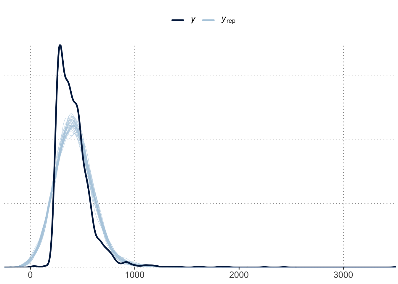
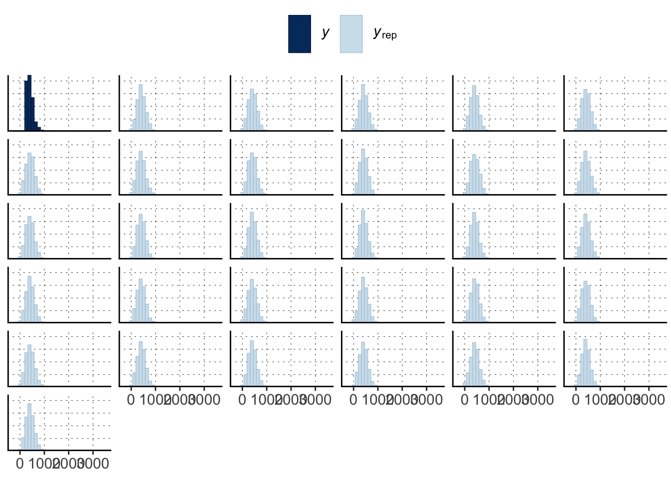
Use tools from the bayesplot package. The basic bayesplot::pp_check() plots the distribution of ndraws samples from the posterior (data) predictive against the distribution of the data the model was trained on:

Toggle code
bayesplot::pp_check(fit_MC, ndraws = 30)

There are many tweaks to pp_check:

Toggle code
bayesplot::pp_check(fit_MC, ndraws = 30, type = "hist")

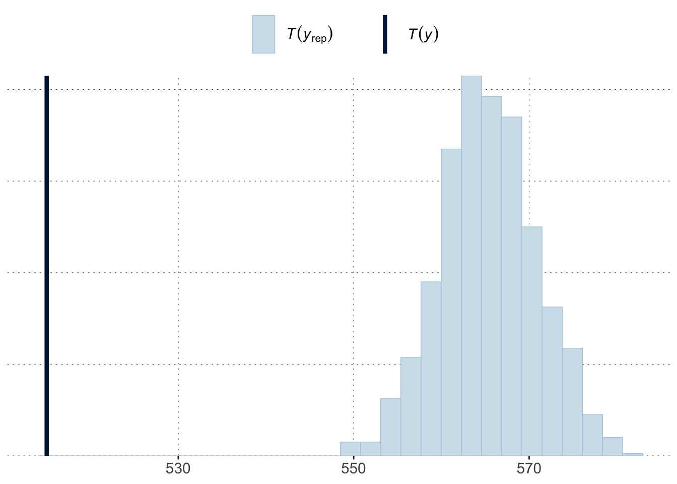
You can also directly use underlying functions like ppc_stat. See help("PPC-overview") and help("PPD-overview") for what is available.

Toggle code
predictive_samples <- brms::posterior_predict(fit_MC, ndraws = 1000)
predictive_samples[1:5, 1:5] 
         [,1]     [,2]     [,3]     [,4]     [,5]
[1,] 299.9574 224.1997 387.6902 534.5947 330.5859
[2,] 305.9095 321.3366 169.0921 340.9020 444.8452
[3,] 347.1188 476.9047 372.1247 181.1809 356.2991
[4,] 269.2256 255.3181 397.9657 250.2674 513.4674
[5,] 429.6383 311.3259 620.8028 241.3073 163.6873
Toggle code
bayesplot::ppc_stat(
  y    = data_MC$RT, 
  yrep = predictive_samples,
  # specify the test statistic of interest
  stat = function(x){quantile(x, 0.8)})

Extracting samples from the posterior predictive distribution

There are three kinds of commonly relevant variables a generalized linear model predicts:

  1. the central tendency of data \(y\) for some predictor \(x\),
  2. the shape of the (hypothetical) data \(y'\) for \(x\), and
  3. a linear predictor value given values of \(x\).

All of these measures can be obtained from a fitted model with different functions, e.g., from the tidyverse package. Here, it does not matter whether the model was fitted to data or it is a “prior model”, so to speak, fit with the flag sample_prior = "only".

Here is an example for a logistic regression model (where all the three measures clearly show their conceptual difference).

Toggle code
fit_MT_logistic <- 
  brms::brm(
    formula = correct ~ group * condition,
    data    = aida::data_MT,
    family  = brms::bernoulli()
  )
Toggle code
# 2 samples from the predicted central tendency
aida::data_MT |> 
  dplyr::select(group, condition) |> 
  unique() |> 
  tidybayes::add_epred_draws(
    fit_MT_logistic,
    ndraws = 2
    )
# A tibble: 8 × 7
# Groups:   group, condition, .row [4]
  group condition  .row .chain .iteration .draw .epred
  <chr> <chr>     <int>  <int>      <int> <int>  <dbl>
1 touch Atypical      1     NA         NA     1  0.917
2 touch Atypical      1     NA         NA     2  0.929
3 touch Typical       2     NA         NA     1  0.932
4 touch Typical       2     NA         NA     2  0.946
5 click Atypical      3     NA         NA     1  0.878
6 click Atypical      3     NA         NA     2  0.851
7 click Typical       4     NA         NA     1  0.963
8 click Typical       4     NA         NA     2  0.961
Toggle code
# 2 samples from the predictive distribution (data samples)
aida::data_MT |> 
  dplyr::select(group, condition) |> 
  unique() |> 
  tidybayes::add_predicted_draws(
    fit_MT_logistic,
    ndraws = 2
    )
# A tibble: 8 × 7
# Groups:   group, condition, .row [4]
  group condition  .row .chain .iteration .draw .prediction
  <chr> <chr>     <int>  <int>      <int> <int>       <int>
1 touch Atypical      1     NA         NA     1           1
2 touch Atypical      1     NA         NA     2           1
3 touch Typical       2     NA         NA     1           1
4 touch Typical       2     NA         NA     2           1
5 click Atypical      3     NA         NA     1           1
6 click Atypical      3     NA         NA     2           0
7 click Typical       4     NA         NA     1           1
8 click Typical       4     NA         NA     2           1
Toggle code
# 2 samples for the linear predictor
aida::data_MT |> 
  dplyr::select(group, condition) |> 
  unique() |> 
  tidybayes::add_linpred_draws(
    fit_MT_logistic,
    ndraws = 2
    )
# A tibble: 8 × 7
# Groups:   group, condition, .row [4]
  group condition  .row .chain .iteration .draw .linpred
  <chr> <chr>     <int>  <int>      <int> <int>    <dbl>
1 touch Atypical      1     NA         NA     1     2.05
2 touch Atypical      1     NA         NA     2     2.77
3 touch Typical       2     NA         NA     1     2.68
4 touch Typical       2     NA         NA     2     2.81
5 click Atypical      3     NA         NA     1     1.80
6 click Atypical      3     NA         NA     2     1.75
7 click Typical       4     NA         NA     1     3.10
8 click Typical       4     NA         NA     2     3.37

Priors

Inspecting default priors without running the model

Toggle code
# define the model as a "brmsformula" object
myFormula <- brms::bf(RT ~ 1 + condition + (1 + condition | submission_id))

# get prior information
brms::get_prior(
  formula = myFormula,
  data    = data_MC,
  family  = exgaussian()
  )
                    prior     class                    coef         group resp
 student_t(3, 385, 133.4) Intercept                                           
                   (flat)         b                                           
                   (flat)         b conditiondiscrimination                   
                   (flat)         b       conditionreaction                   
            gamma(1, 0.1)      beta                                           
                   lkj(1)       cor                                           
                   lkj(1)       cor                         submission_id     
   student_t(3, 0, 133.4)        sd                                           
   student_t(3, 0, 133.4)        sd                         submission_id     
   student_t(3, 0, 133.4)        sd               Intercept submission_id     
   student_t(3, 0, 133.4)        sd conditiondiscrimination submission_id     
   student_t(3, 0, 133.4)        sd       conditionreaction submission_id     
   student_t(3, 0, 133.4)     sigma                                           
 dpar nlpar lb ub       source
                       default
                       default
                  (vectorized)
                  (vectorized)
             0         default
                       default
                  (vectorized)
             0         default
             0    (vectorized)
             0    (vectorized)
             0    (vectorized)
             0    (vectorized)
             0         default

Setting priors

Toggle code
myPrior <- 
  brms::prior("normal(30,100)",  class = "b", coef = "conditiondiscrimination") +
  brms::prior("normal(-30,100)", class = "b", coef = "conditionreaction")

fit_with_specified_prior <- 
  brms::brm(
    formula = myformula,
    data    = data_MC,
    prior   = myPrior,
    family  = exgaussian()
  )

Sampling from the prior

Toggle code
fit_samples_from_prior_only <- 
brms::brm(
  formula = myformula,
  data    = data_MC,
  prior   = myPrior,
  family  = exgaussian(),
  sample_prior = "only"
)

Under the hood: Stan code, design matrices etc.

Extract the Stan code

Toggle code
brms::stancode(fit_MC)
// generated with brms 2.20.1
functions {
 /* compute correlated group-level effects
  * Args:
  *   z: matrix of unscaled group-level effects
  *   SD: vector of standard deviation parameters
  *   L: cholesky factor correlation matrix
  * Returns:
  *   matrix of scaled group-level effects
  */
  matrix scale_r_cor(matrix z, vector SD, matrix L) {
    // r is stored in another dimension order than z
    return transpose(diag_pre_multiply(SD, L) * z);
  }
}
data {
  int<lower=1> N;  // total number of observations
  vector[N] Y;  // response variable
  int<lower=1> K;  // number of population-level effects
  matrix[N, K] X;  // population-level design matrix
  int<lower=1> Kc;  // number of population-level effects after centering
  // data for group-level effects of ID 1
  int<lower=1> N_1;  // number of grouping levels
  int<lower=1> M_1;  // number of coefficients per level
  int<lower=1> J_1[N];  // grouping indicator per observation
  // group-level predictor values
  vector[N] Z_1_1;
  vector[N] Z_1_2;
  vector[N] Z_1_3;
  vector[N] Z_1_4;
  int<lower=1> NC_1;  // number of group-level correlations
  int prior_only;  // should the likelihood be ignored?
}
transformed data {
  matrix[N, Kc] Xc;  // centered version of X without an intercept
  vector[Kc] means_X;  // column means of X before centering
  for (i in 2:K) {
    means_X[i - 1] = mean(X[, i]);
    Xc[, i - 1] = X[, i] - means_X[i - 1];
  }
}
parameters {
  vector[Kc] b;  // regression coefficients
  real Intercept;  // temporary intercept for centered predictors
  real<lower=0> sigma;  // dispersion parameter
  vector<lower=0>[M_1] sd_1;  // group-level standard deviations
  matrix[M_1, N_1] z_1;  // standardized group-level effects
  cholesky_factor_corr[M_1] L_1;  // cholesky factor of correlation matrix
}
transformed parameters {
  matrix[N_1, M_1] r_1;  // actual group-level effects
  // using vectors speeds up indexing in loops
  vector[N_1] r_1_1;
  vector[N_1] r_1_2;
  vector[N_1] r_1_3;
  vector[N_1] r_1_4;
  real lprior = 0;  // prior contributions to the log posterior
  // compute actual group-level effects
  r_1 = scale_r_cor(z_1, sd_1, L_1);
  r_1_1 = r_1[, 1];
  r_1_2 = r_1[, 2];
  r_1_3 = r_1[, 3];
  r_1_4 = r_1[, 4];
  lprior += student_t_lpdf(Intercept | 3, 385, 133.4);
  lprior += student_t_lpdf(sigma | 3, 0, 133.4)
    - 1 * student_t_lccdf(0 | 3, 0, 133.4);
  lprior += student_t_lpdf(sd_1 | 3, 0, 133.4)
    - 4 * student_t_lccdf(0 | 3, 0, 133.4);
  lprior += lkj_corr_cholesky_lpdf(L_1 | 1);
}
model {
  // likelihood including constants
  if (!prior_only) {
    // initialize linear predictor term
    vector[N] mu = rep_vector(0.0, N);
    mu += Intercept;
    for (n in 1:N) {
      // add more terms to the linear predictor
      mu[n] += r_1_1[J_1[n]] * Z_1_1[n] + r_1_2[J_1[n]] * Z_1_2[n] + r_1_3[J_1[n]] * Z_1_3[n] + r_1_4[J_1[n]] * Z_1_4[n];
    }
    target += normal_id_glm_lpdf(Y | Xc, mu, b, sigma);
  }
  // priors including constants
  target += lprior;
  target += std_normal_lpdf(to_vector(z_1));
}
generated quantities {
  // actual population-level intercept
  real b_Intercept = Intercept - dot_product(means_X, b);
  // compute group-level correlations
  corr_matrix[M_1] Cor_1 = multiply_lower_tri_self_transpose(L_1);
  vector<lower=-1,upper=1>[NC_1] cor_1;
  // extract upper diagonal of correlation matrix
  for (k in 1:M_1) {
    for (j in 1:(k - 1)) {
      cor_1[choose(k - 1, 2) + j] = Cor_1[j, k];
    }
  }
}

Extract Stan data

This is the data passed to Stan. Useful for inspecting dimensions etc.

Toggle code
brms::standata(fit_MC) |> names()
 [1] "N"          "Y"          "K"          "Kc"         "X"         
 [6] "Z_1_1"      "Z_1_2"      "Z_1_3"      "Z_1_4"      "J_1"       
[11] "N_1"        "M_1"        "NC_1"       "prior_only"

Inspect design matrices

Population-level effects

Toggle code
X <- brms::standata(fit_MC)$X
X |> head()
  Intercept conditionreaction conditiondiscrimination
1         1                 1                       0
2         1                 1                       0
3         1                 1                       0
4         1                 1                       0
5         1                 1                       0
6         1                 1                       0

Group-level effects

The group-level design matrix is spread out over different variables (all names Z_ followed by some indices), but retrievable like so:

Toggle code
data4Stan <- brms::standata(fit_MC)
Z <- data4Stan[str_detect(data4Stan |> names(), "Z_")] |> as_tibble()
Z
# A tibble: 2,519 × 4
       Z_1_1     Z_1_2     Z_1_3     Z_1_4
   <dbl[1d]> <dbl[1d]> <dbl[1d]> <dbl[1d]>
 1         1         1         0         0
 2         1         1         0         1
 3         1         1         0         1
 4         1         1         0         1
 5         1         1         0         0
 6         1         1         0         1
 7         1         1         0         1
 8         1         1         0         0
 9         1         1         0         1
10         1         1         0         0
# ℹ 2,509 more rows