Bayesian regression models in WebPPL

Bayesian regression: theory & practice

Preamble

Here is code to load (and if necessary, install) required packages, and to set some global options (for plotting and efficient fitting of Bayesian models).

Toggle code

# install packages from CRAN (unless installed)
pckgs_needed <- c(
  "tidyverse",
  "brms",
  "rstan",
  "rstanarm",
  "remotes",
  "tidybayes",
  "bridgesampling",
  "shinystan",
  "mgcv"
)
pckgs_installed <- installed.packages()[,"Package"]
pckgs_2_install <- pckgs_needed[!(pckgs_needed %in% pckgs_installed)]
if(length(pckgs_2_install)) {
  install.packages(pckgs_2_install)
} 

# install additional packages from GitHub (unless installed)
if (! "aida" %in% pckgs_installed) {
  remotes::install_github("michael-franke/aida-package")
}
if (! "faintr" %in% pckgs_installed) {
  remotes::install_github("michael-franke/faintr")
}
if (! "cspplot" %in% pckgs_installed) {
  remotes::install_github("CogSciPrag/cspplot")
}

# load the required packages
x <- lapply(pckgs_needed, library, character.only = TRUE)
library(aida)
library(faintr)
library(cspplot)

# these options help Stan run faster
options(mc.cores = parallel::detectCores())

# use the CSP-theme for plotting
theme_set(theme_csp())

# global color scheme from CSP
project_colors = cspplot::list_colors() |> pull(hex)
# names(project_colors) <- cspplot::list_colors() |> pull(name)

# setting theme colors globally
scale_colour_discrete <- function(...) {
  scale_colour_manual(..., values = project_colors)
}
scale_fill_discrete <- function(...) {
   scale_fill_manual(..., values = project_colors)
}

Simple regression

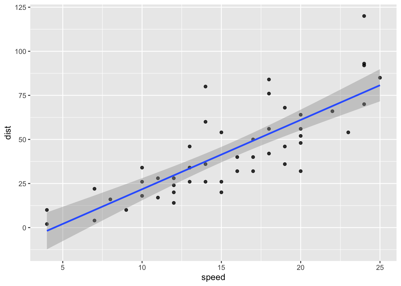
Let’s loot at R’s built-in data set cars for simple example of two paired metric measurements. Here, we have the speed a car was traveling and the distance before coming to a halt (from the 1920s):

Toggle code

cars |> 
  ggplot(aes(x = speed, y = dist)) +
  geom_point(alpha = 0.8) +
  geom_smooth(method = "lm")

Here is an example of a simple Bayesian regression model for this data set in WebPPL.

// R's 'cars' data set: 50 paired measurements of speed and distance (after breaking)
var speed = [4, 4, 7, 7, 8, 9, 10, 10, 
             10, 11, 11, 12, 12, 12, 
             12, 13, 13, 13, 13, 14, 
             14, 14, 14, 15, 15, 15, 
             16, 16, 17, 17, 17, 18, 
             18, 18, 18, 19, 19, 19, 
             20, 20, 20, 20, 20, 22, 
             23, 24, 24, 24, 24, 25]
var dist = [2, 10, 4, 22, 16, 10, 18, 
            26, 34, 17, 28, 14, 20, 24, 
            28, 26, 34, 34, 46, 26, 36, 
            60, 80, 20, 26, 54, 32, 40, 
            32, 40, 50, 42, 56, 76, 84, 
            36, 46, 68, 32, 48, 52, 56, 
            64, 66, 54, 70, 92, 93, 120, 85]

var model = function() {
  
  // parameters & priors
  var Intercept = gaussian(-18, 5); // data-informed choice (!)
  var slope = gaussian(0, 10);
  var sigma = gamma(5, 5);

  // linear predictor value for a given 'x' value
  var linPred = function(x) {
    return slope * x + Intercept;
  };

  map2(
    function(x, y) {
      factor(Gaussian({mu: linPred(x), sigma: sigma}).score(y));
    },
    speed,
    dist);

  return {Intercept,slope, sigma};
}

viz.marginals(Infer({method: 'MCMC', samples: 20000, burn: 10000, lag: 2}, model));

Exercise 1

1. Try to see the underlying model of the data-generating process behind the code.
2. Visualize just the priors and compare them with the posteriors.
3. Why is it (usually!) okay to glimpse at the data to set priors for the Intercept?

Solution

Usually, it is the slope coefficients that capture the research question of interest. We should therefore (usually) be more mindful about setting the priors for the slope coefficients.

Linear regression for A/B testing

Here is an example in WebPPL of an application of a linear regression model to a case of A/B-testing, i.e., investigating whether there is a difference between two sets of measurements. If we encode the difference between groups as a slope coefficient, we can use the linear regression format to, essentially, mimick a kind of t-test (with unpaired measurements and equal variance).

var y_A = [127, 130, 106, 129, 114, 125, 119, 128]
var y_B = [131, 119, 115, 109, 110, 105, 118, 112]

// define likelihood function
var LH_fun = function(mu, sigma, y_obs) {
  map(
    function(y) {var LH = Gaussian({mu: mu, sigma: sigma}).score(y);
                 factor(LH);},
    y_obs );
}

var model = function() {
  // model parameters
  var beta_0 = gaussian(120,50);
  var beta_1 = gaussian(0,30);
  var sigma  = gamma(5,5);

  // linear predictor (= predictor of central tendency)
  var mu_A = beta_0
  var mu_B = beta_0 + beta_1

  // apply likelihood function
  LH_fun(mu_A, sigma, y_A);
  LH_fun(mu_B, sigma, y_B);

  // samples from the posterior predictive distribution
//   var y_A_pred = gaussian(mu_A, sigma)
//   var y_B_pred = gaussian(mu_B, sigma)

  return {beta_0, beta_1, sigma};
//   return {y_A_pred , y_B_pred}
  
}

viz.marginals(Infer({method: 'MCMC', samples: 15000, lag: 2, burn: 5000}, model));

Exercise 2

1. Try to see the underlying model of the data-generating process behind the code.
2. Visualize just the priors and compare them with the posteriors.
3. Use the commented-out code to draw samples from the posterior predictive distribution.
4. Now draw samples from the prior predictive distribution.
5. If you wanted to mimick a t-test with unequal variance instead, could you change the code to do that? (NB: we only have very few data points, so your posteriors will likely be quite “ragged”.)