This tutorial discusses a minimal example of a mixture model. After introducing the main idea behind mixture models, a fictitious (minimal) data set is analyzed first with a hand-written Stan program, and then with a mixture regression model using brms.
Preamble
Here is code to load (and if necessary, install) required packages, and to set some global options (for plotting and efficient fitting of Bayesian models).
Toggle code
# install packages from CRAN (unless installed)pckgs_needed <-c("tidyverse","brms","rstan","rstanarm","remotes","tidybayes","bridgesampling","shinystan","mgcv")pckgs_installed <-installed.packages()[,"Package"]pckgs_2_install <- pckgs_needed[!(pckgs_needed %in% pckgs_installed)]if(length(pckgs_2_install)) {install.packages(pckgs_2_install)} # install additional packages from GitHub (unless installed)if (!"aida"%in% pckgs_installed) { remotes::install_github("michael-franke/aida-package")}if (!"faintr"%in% pckgs_installed) { remotes::install_github("michael-franke/faintr")}if (!"cspplot"%in% pckgs_installed) { remotes::install_github("CogSciPrag/cspplot")}# load the required packagesx <-lapply(pckgs_needed, library, character.only =TRUE)library(aida)library(faintr)library(cspplot)# these options help Stan run fasteroptions(mc.cores = parallel::detectCores())# use the CSP-theme for plottingtheme_set(theme_csp())# global color scheme from CSPproject_colors = cspplot::list_colors() |>pull(hex)# names(project_colors) <- cspplot::list_colors() |> pull(name)# setting theme colors globallyscale_colour_discrete <-function(...) {scale_colour_manual(..., values = project_colors)}scale_fill_discrete <-function(...) {scale_fill_manual(..., values = project_colors)}
Finite mixtures: Motivation & set-up
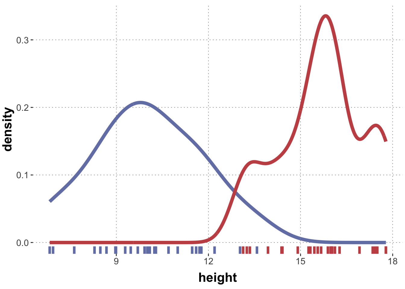
To motivate mixture modeling, let’s look at a fictitious data set. There are two sets of measurements. For each of two species of plants, we measured the length of 25 exemplars.
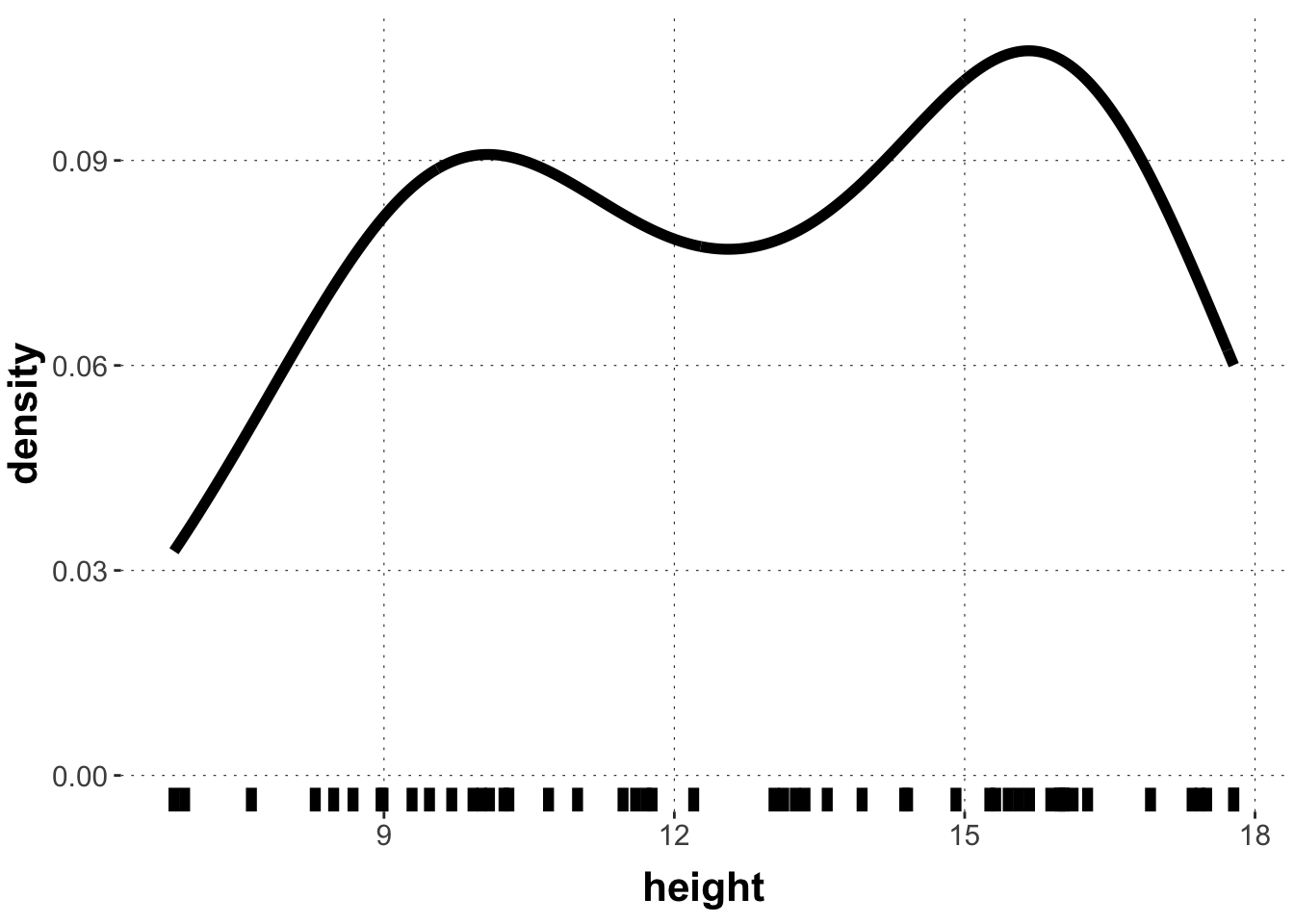
Now suppose that (for whatever reason) we get the data without information which measure was from which group. If we plot the data without this information, the picture looks like this:
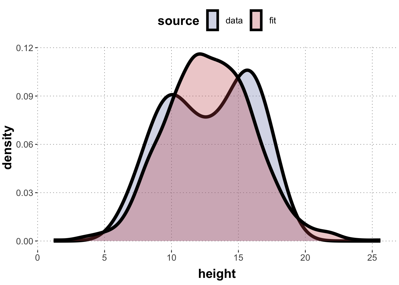
Data may often look like this, showing signs of bi- or multi-modality, i.e., having several “humps” or apparent local areas of higher concentration. If we fit a single Gaussian to this data it might look like this:
Toggle code
# using the descriptive means/SD for a quick "best fit"mu <-mean(flower_heights)sigma <-sd(flower_heights)tibble(source =c(rep("data", length(flower_heights)), rep("fit", 1000)),height =c(flower_heights, rnorm(1000, mu, sigma))) |>ggplot(aes(x = height, fill=source)) +geom_density(size =2, alpha =0.3)
If we see a posterior predictive check that looks like this picture above, you know that there is something systematic amiss with your model: you assume a single peak (a multimodal response distribution) but the data shows signs of multi-modality (several “peaks” or centers of high density).
Models that allow multiple “peaks” in the response distribution, are mixture models. When dealing with a Gaussian likelihood function, as in the case at hand, we speak of Gaussian mixture models (GMM). In general, a mixture model incorporates the idea that the data was generated from more than one process (alternative lingo: that observations were samples from different populations).
Let \(\langle f_1, \dots, f_k \rangle\) be \(k\) likelihood functions for data \(Y\). The \(k\)-mixture model for \(Y\) explains the data as a weighted combination, with mixture weights \(\alpha\) (a probability vector). Procedurally, think of inferring for each data point \(y_{i}\) which a mixture component \(k(i)\) most likelihood belongs to (i.e., by which of \(k\) different processes it may have been generated; or, from which of \(k\) different populations it was sampled). The probability that any \(y_{i}\) is in class \(j\) is given by \(\alpha_{i}\), so that \(\alpha\) represents the overall probabilities of different components (sub-populations). This results in a mixture likelihood function which can be written like so:
\[f^{\mathrm{MM}}(y_i) = \alpha_{k(i)} f_{k(i)}\]
For the current case, we assume that there are just two components (because we see two “humps”, or have a priori information that there are exactly two groups. Concretely, for each data point \(y_i\), \(i \in \{1, \dots, N\}\), we are going to estimate how likely data point \(i\) may have been a sample from normal distribution “Number 0”, with \(\mu_0\) and \(\sigma_0\), or from normal distribution “Number 1”, with \(\mu_1\) and \(\sigma_1\). Naturally, all \(\mu_{0,1}\) and \(\sigma_{0,1}\) are estimated from the data, as are the group-indicator variables \(z_i\). There is also a global parameter \(p\) which indicates how likely any data point is to come from one of the two distributions (you’ll think about which one below!). Here’s the full model we will work with (modulo an additional ordering constraint, as discussed below):
Below is the Stan code for this model. It is also given in file Gaussian-mixture-01-basic.stan. A few comments on this code:
There is no occurrence of variable \(z_i\), as this is marginalized out. We do this by incrementing the log-score manually, using target += log_sum_exp(alpha).
We declare vector mu to be of a particular type which we have not seen before. We want the vector to be ordered. We will come back to this later. Don’t worry about it now.
data {int<lower=1> N; real y[N]; }parameters {real<lower=0,upper=1> p; ordered[2] mu; vector<lower=0>[2] sigma; }model { p ~ beta(1,1); mu ~ normal(12, 10); sigma ~ lognormal(0, 1);for (i in1:N) {vector[2] alpha; alpha[1] = log(p) + normal_lpdf(y[i] | mu[1], sigma[1]); alpha[2] = log(1-p) + normal_lpdf(y[i] | mu[2], sigma[2]);target += log_sum_exp(alpha); }}
Inference for Stan model: anon_model.
4 chains, each with iter=2000; warmup=1000; thin=1;
post-warmup draws per chain=1000, total post-warmup draws=4000.

            mean se_mean   sd    2.5%     25%     50%     75%   97.5% n_eff
p           0.54    0.01 0.14    0.25    0.45    0.55    0.63    0.83   625
mu[1]      10.38    0.04 0.93    8.85    9.80   10.35   10.93   12.32   646
mu[2]      15.70    0.03 0.67   13.94   15.41   15.79   16.12   16.67   452
sigma[1]    2.07    0.02 0.60    1.10    1.65    2.02    2.45    3.37   873
sigma[2]    1.41    0.02 0.50    0.71    1.08    1.33    1.63    2.84   504
lp__     -127.33    0.12 2.20 -133.41 -128.27 -126.76 -125.81 -124.79   350
         Rhat
p        1.01
mu[1]    1.01
mu[2]    1.00
sigma[1] 1.00
sigma[2] 1.01
lp__     1.00

Samples were drawn using NUTS(diag_e) at Wed Mar  5 13:56:12 2025.
For each parameter, n_eff is a crude measure of effective sample size,
and Rhat is the potential scale reduction factor on split chains (at
convergence, Rhat=1).
Exercise 1b: Interpret this outcome
Interpret these results! Focus on parameters \(p\), \(\mu_1\) and \(\mu_2\). What does \(p\) capture in this implementation? Do the (mean) estimated values make sense?
Solution
Yes, they do make sense. \(p\) is the prevalence of data from the group with the higher mean, which is group \(B\) in our case. The model infers that there are roughly equally many data points from each group, which is indeed the case. The model also recovers the descriptive means of each group!
# A tibble: 2 × 3
  species  mean std_dev
  <chr>   <dbl>   <dbl>
1 A        10.0    1.76
2 B        15.7    1.38
An unidentifiable model
Let’s run the model in file Gaussian-mixture-02-unindentifiable.stan, which is exactly the same as before but with vector mu being an unordered vector of reals.
Toggle code
stan_fit_2c_GMM <-stan(file ='stan-files/Gaussian-mixture-02-unindentifiable.stan',data = data_GMM,# set a seed for reproducible resultsseed =1734)
Here’s a summary of the outcome:
Toggle code
stan_fit_2c_GMM
Inference for Stan model: anon_model.
4 chains, each with iter=2000; warmup=1000; thin=1;
post-warmup draws per chain=1000, total post-warmup draws=4000.

            mean se_mean   sd    2.5%     25%     50%     75%   97.5% n_eff
p           0.50    0.02 0.14    0.21    0.40    0.50    0.59    0.77    81
mu[1]      12.85    1.80 2.77    9.13   10.20   11.71   15.72   16.50     2
mu[2]      13.26    1.75 2.77    9.19   10.44   14.76   15.82   16.50     3
sigma[1]    1.75    0.21 0.61    0.80    1.30    1.66    2.12    3.11     8
sigma[2]    1.74    0.21 0.64    0.80    1.27    1.64    2.10    3.18     9
lp__     -128.86    0.05 1.86 -133.37 -129.79 -128.46 -127.51 -126.51  1241
         Rhat
p        1.04
mu[1]    2.72
mu[2]    2.41
sigma[1] 1.18
sigma[2] 1.16
lp__     1.00

Samples were drawn using NUTS(diag_e) at Wed Mar  5 13:56:32 2025.
For each parameter, n_eff is a crude measure of effective sample size,
and Rhat is the potential scale reduction factor on split chains (at
convergence, Rhat=1).
Exercise 1c: Interpret model output
What is remarkable here? Explain what happened. Explain in what sense this model is “unidentifiable”.
Hint: Explore the parameters with high \(\hat{R}\) values. When a model fit seems problematic, a nice tool to explore what might be amiss is the package shinystan. You could do this:
Toggle code
shinystan::launch_shinystan(stan_fit_2c_GMM)
Then head over to the tab “Explore” and have a look at some of the parameters.
Solution
The \(\hat{R}\) values of the mean parameters are substantially above 1, suggesting that the model did not converge. But if we look at trace plots for these parameters, for example, we see that \(\mu_1\) has “locked into” group A for some chains, and into group B for some other chains.
The model is therefore unidentifiable in the sense that, without requiring that mu is ordered, \(\mu_1\) could be for group A or group B, and which one it will take on depends on random initialization. Requiring that mu be ordered, breaks this symmetry.
Posterior predictive check
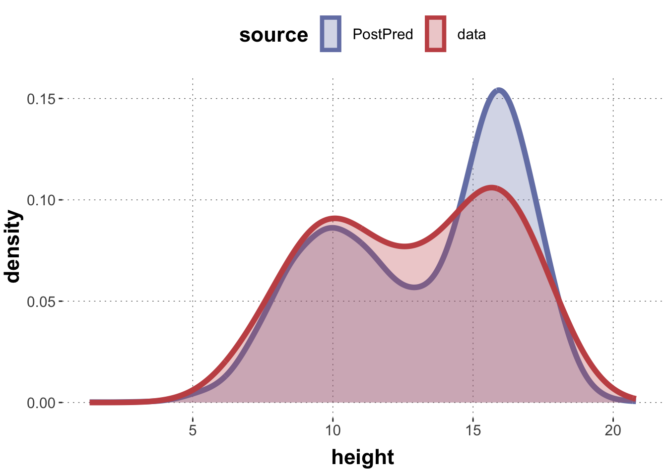
We can extend the (identifiable) model from above to also output samples from the posterior predictive distribution. This is given in file Gaussian-mixture-03-withPostPred.stan. Let’s run this model, collect the posterior predictive samples in a variable called yrep and draw a density plot.
Toggle code
stan_fit_2d_GMM <-stan(file ='stan-files/Gaussian-mixture-03-withPostPred.stan',data = data_GMM,# only return the posterior predictive samplespars =c('yrep'))
Does this look like a distribution that could have generated the data?
Solution
The distribution looks plausible enough. The visual fit in these density plots is not perfect also because we use quite a different number of samples to estimate the density.
A Gaussian mixture model in brms
We can also run this finite mixture model in brms. Fitting the parameters of a single Gaussian is like fitting an intercept-only simple linear regression model. We can add finite mixtures to brms via the family parameter and the function brms::mixture(). Here, we define a finite mixture of Gaussians, of course, but more flexibility is possible.
Toggle code
brms_fit_2e_GMM <-brm(# intercept only modelformula = y ~1, data = data_GMM, # declare that the likelihood should be a mixturefamily =mixture(gaussian, gaussian),# use weakly informative priors on mu prior =c(prior(normal(12, 10), Intercept, dpar = mu1),prior(normal(12, 10), Intercept, dpar = mu2) ))
Let’s look at the model fit:
Toggle code
brms_fit_2e_GMM
 Family: mixture(gaussian, gaussian)
  Links: mu1 = identity; sigma1 = identity; mu2 = identity; sigma2 = identity; theta1 = identity; theta2 = identity
Formula: y ~ 1
   Data: data_GMM (Number of observations: 50)
  Draws: 4 chains, each with iter = 2000; warmup = 1000; thin = 1;
         total post-warmup draws = 4000

Population-Level Effects:
              Estimate Est.Error l-95% CI u-95% CI Rhat Bulk_ESS Tail_ESS
mu1_Intercept    10.47      1.00     8.89    12.59 1.00      723      643
mu2_Intercept    15.69      1.17    13.47    16.76 1.01      755      418

Family Specific Parameters:
       Estimate Est.Error l-95% CI u-95% CI Rhat Bulk_ESS Tail_ESS
sigma1     2.24      0.68     1.19     3.60 1.00      785     1179
sigma2     1.58      0.98     0.76     3.27 1.00      877      505
theta1     0.54      0.16     0.19     0.88 1.01      722      565
theta2     0.46      0.16     0.12     0.81 1.01      722      565

Draws were sampled using sampling(NUTS). For each parameter, Bulk_ESS
and Tail_ESS are effective sample size measures, and Rhat is the potential
scale reduction factor on split chains (at convergence, Rhat = 1).
Let’s also look at the Stan code that brms produced in the background for this model in order to find out how this model is related to that of Ex 2.b:
Toggle code
brms_fit_2e_GMM$model
// generated with brms 2.20.1
functions {
}
data {
  int<lower=1> N;  // total number of observations
  vector[N] Y;  // response variable
  vector[2] con_theta;  // prior concentration
  int prior_only;  // should the likelihood be ignored?
}
transformed data {
}
parameters {
  real<lower=0> sigma1;  // dispersion parameter
  real<lower=0> sigma2;  // dispersion parameter
  simplex[2] theta;  // mixing proportions
  ordered[2] ordered_Intercept;  // to identify mixtures
}
transformed parameters {
  // identify mixtures via ordering of the intercepts
  real Intercept_mu1 = ordered_Intercept[1];
  // identify mixtures via ordering of the intercepts
  real Intercept_mu2 = ordered_Intercept[2];
  // mixing proportions
  real<lower=0,upper=1> theta1;
  real<lower=0,upper=1> theta2;
  real lprior = 0;  // prior contributions to the log posterior
  theta1 = theta[1];
  theta2 = theta[2];
  lprior += normal_lpdf(Intercept_mu1 | 12, 10);
  lprior += student_t_lpdf(sigma1 | 3, 0, 4.2)
    - 1 * student_t_lccdf(0 | 3, 0, 4.2);
  lprior += normal_lpdf(Intercept_mu2 | 12, 10);
  lprior += student_t_lpdf(sigma2 | 3, 0, 4.2)
    - 1 * student_t_lccdf(0 | 3, 0, 4.2);
  lprior += dirichlet_lpdf(theta | con_theta);
}
model {
  // likelihood including constants
  if (!prior_only) {
    // initialize linear predictor term
    vector[N] mu1 = rep_vector(0.0, N);
    // initialize linear predictor term
    vector[N] mu2 = rep_vector(0.0, N);
    mu1 += Intercept_mu1;
    mu2 += Intercept_mu2;
    // likelihood of the mixture model
    for (n in 1:N) {
      real ps[2];
      ps[1] = log(theta1) + normal_lpdf(Y[n] | mu1[n], sigma1);
      ps[2] = log(theta2) + normal_lpdf(Y[n] | mu2[n], sigma2);
      target += log_sum_exp(ps);
    }
  }
  // priors including constants
  target += lprior;
}
generated quantities {
  // actual population-level intercept
  real b_mu1_Intercept = Intercept_mu1;
  // actual population-level intercept
  real b_mu2_Intercept = Intercept_mu2;
}
Now, your job. Look at the two previous outputs and answer the following questions:
Exercise 2a
Is the brms-model the exact same as the model in the previous section (model coded directly in Stan)?
Solution
No, the priors on \(\mu\) and \(\sigma\) are different.
Exercise 2b
What is the equivalent of the variable alpha from the model of the previous section in this new brms-generated code?
Solution
That’s ps
Exercise 2c
What is the equivalent of the variable p from the model of Ex 2.b in this new brms-generated code?
Solution
That’s theta[1]
Exercise 2d
Is the brms code generating posterior predictive samples?
Solution
No! This is not strictly necessary. These can be generated also later for a fitted object.
Exercise 2e
What is the prior probability in the brms-generated model of any given data point \(y_i\) to be from the first or second mixture component? Can you even tell from the code?
Solution
We cannot say. It’s in the variable con_theta but that is supplied from the outside. We can only guess. (A good guess would be: yes, it’s also unbiased 50/50.)