05b: Hierarchical regression models (exercises)

Bayesian regression: theory & practice

Author

Michael Franke & Timo Roettger

Preamble

Here is code to load (and if necessary, install) required packages, and to set some global options (for plotting and efficient fitting of Bayesian models).

Toggle code

# install packages from CRAN (unless installed)
pckgs_needed <- c(
  "tidyverse",
  "brms",
  "rstan",
  "rstanarm",
  "remotes",
  "tidybayes",
  "bridgesampling",
  "shinystan",
  "mgcv"
)
pckgs_installed <- installed.packages()[,"Package"]
pckgs_2_install <- pckgs_needed[!(pckgs_needed %in% pckgs_installed)]
if(length(pckgs_2_install)) {
  install.packages(pckgs_2_install)
} 

# install additional packages from GitHub (unless installed)
if (! "aida" %in% pckgs_installed) {
  remotes::install_github("michael-franke/aida-package")
}
if (! "faintr" %in% pckgs_installed) {
  remotes::install_github("michael-franke/faintr")
}
if (! "cspplot" %in% pckgs_installed) {
  remotes::install_github("CogSciPrag/cspplot")
}

# load the required packages
x <- lapply(pckgs_needed, library, character.only = TRUE)
library(aida)
library(faintr)
library(cspplot)

# these options help Stan run faster
options(mc.cores = parallel::detectCores())

# use the CSP-theme for plotting
theme_set(theme_csp())

# global color scheme from CSP
project_colors = cspplot::list_colors() |> pull(hex)
# names(project_colors) <- cspplot::list_colors() |> pull(name)

# setting theme colors globally
scale_colour_discrete <- function(...) {
  scale_colour_manual(..., values = project_colors)
}
scale_fill_discrete <- function(...) {
   scale_fill_manual(..., values = project_colors)
}

Toggle code

dolphin <- aida::data_MT
my_scale <- function(x) c(scale(x))

Exercise 1: Logistic regression

Consider the following model formula for the dolphin data set:

Toggle code

brms::bf(MAD ~ condition + 
     (condition || subject_id) +
     (condition || exemplar))

MAD ~ condition + (condition || subject_id) + (condition || exemplar)

Exercise 1a

Why is the random effect structure of this model questionable? Can we meaningfully estimate all parameters? (Hint: Think about what group levels vary across predictor levels)

Solution

Factor condition is not crossed with exemplar. An exemplar is either typical or atypical, thus a random slope does not make sense.

Exercise 1b

Use the following data frame:

Toggle code

# set up data frame
dolphin_correct <- dolphin %>% 
  filter(correct == 1) %>% 
  mutate(log_RT_s = my_scale(log(RT)),
         AUC_s = my_scale(AUC))

Run a multilevel model that predicts AUC_s based on condition. Specify maximal random effect structures for exemplars and subject_ids (ignore correlations between intercepts and slopes for now). Specify a seed = 98.

If you encounter “divergent transition” warning, make them go away by refitting the model appropriately (Hint: brms gives very useful, actionable advice)

(This might take a couple of minutes, get used to it ;)

Solution

Toggle code

# refit with upped adapt_delta and max_treedepth
xmdl_AUC2 <- brm(AUC_s ~ condition +
                  (condition || subject_id) +
                  (1 | exemplar),
                data = dolphin_correct,
                control=list(adapt_delta=0.99, max_treedepth=15), 
                seed = 98
                )
xmdl_AUC2

Exercise 1c

You want to run a multilevel model that predicts log_RT_s based on group. You want to account for group-level variation of both subject_id and exemplar. What kind of groupings can be meaningfully estimated, given the dataset and the experimental design. You can check the crossing of different vectors with xtabs() for example.

Solution

Toggle code

# check crossing
xtabs(~ group + subject_id, dolphin_correct)

       subject_id
group   1001 1002 1003 1004 1005 1006 1007 1008 1009 1010 1011 1012 1013 1014
  click    0   19   17    0    0    0   19    0    0   19    0    0   17   16
  touch   16    0    0   18   17   19    0   18   19    0   19   16    0    0
       subject_id
group   1015 1016 1017 1018 1019 1020 1021 1022 1023 1024 1025 1026 1027 1028
  click   18    0    0    0   19   17    0   19   14    0    0   19    0   19
  touch    0   18   19   17    0    0   18    0    0   19   12    0   17    0
       subject_id
group   1029 1030 1031 1032 1033 1034 1035 1036 1037 1038 1039 1040 1041 1042
  click    0   19   15    0   17   19    0    0   18    0   19    0   17    0
  touch   19    0    0   19    0    0   19   16    0   17    0   18    0   18
       subject_id
group   1043 1044 1045 1046 1047 1048 1049 1050 1051 1052 1053 1054 1055 1056
  click    0   17   17   18    0   18   17   18    0    0    0    0   18    0
  touch   19    0    0    0   19    0    0    0   18   17   18   19    0   19
       subject_id
group   1057 1058 1059 1060 1061 1062 1063 1064 1065 1066 1067 1068 1069 1070
  click    0    0   18   18   17    0   16   17    0   18    0   17    0   18
  touch   19   18    0    0    0   19    0    0   18    0   18    0   17    0
       subject_id
group   1071 1072 1073 1074 1075 1076 1077 1078 1079 1080 1081 1082 1083 1084
  click   19   19    0   19    0   19    0   19   19    0    0    0   18   19
  touch    0    0   15    0   19    0   19    0    0   19   17   15    0    0
       subject_id
group   1085 1086 1087 1088 1089 1090 1091 1092 1093 1094 1095 1096 1097 1098
  click   19    0    0   18    0    0   18    0    0    0   19   15    0    0
  touch    0   11   17    0   19   18    0   19   18   15    0    0   19   17
       subject_id
group   1099 1100 1101 1102 1103 1104 1105 1106 1107 1108
  click   16    0   18    0    0   14   19    0   17    0
  touch    0   19    0   18   17    0    0   19    0   17

Toggle code

# individual subject_ids contributed data only to one group because it is a between-subject design
# --> we need varying intercepts only, i.e. a different base-rate for subjects

xtabs(~ group + exemplar, dolphin_correct)

       exemplar
group   alligator bat butterfly cat chameleon dog eel goldfish hawk horse lion
  click        51  38        52  53        52  53  50       53   53    53   53
  touch        53  46        54  54        54  53  53       55   52    53   54
       exemplar
group   penguin rabbit rattlesnake salmon sealion shark sparrow whale
  click      48     53          38     53      48    46      53    42
  touch      52     51          43     52      50    44      55    45

Toggle code

# each exemplar contributes data to both groups
# --> we can integrate varying intercepts and slopes for exemplars

Exercise 1d

Run a multilevel model that predicts log_RT_s based on group and add maximal random effect structures licensed by the experimental design (ignore possible random intercept-slope interactions for now).

Specify weakly informative priors as you see fit.

Solution

Toggle code

priors <- c(
  #priors for all fixed effects (group)
  set_prior("student_t(3, 0, 3)", class = "b"),
  #prior for the Intercept
  set_prior("student_t(3, 0, 3)", class = "Intercept"),
  #prior for all SDs including the varying intercepts and slopes
  set_prior("student_t(3, 0, 3)", class = "sd")
)

xmdl <- brm(log_RT_s ~ group + 
              (1 | subject_id) +
              (group || exemplar),
            prior = priors,
            data = dolphin_correct)
xmdl

 Family: gaussian 
  Links: mu = identity; sigma = identity 
Formula: log_RT_s ~ group + (1 | subject_id) + (group || exemplar) 
   Data: dolphin_correct (Number of observations: 1915) 
  Draws: 4 chains, each with iter = 2000; warmup = 1000; thin = 1;
         total post-warmup draws = 4000

Group-Level Effects: 
~exemplar (Number of levels: 19) 
               Estimate Est.Error l-95% CI u-95% CI Rhat Bulk_ESS Tail_ESS
sd(Intercept)      0.45      0.09     0.32     0.65 1.00      778     1525
sd(grouptouch)     0.11      0.06     0.01     0.23 1.00      890      890

~subject_id (Number of levels: 108) 
              Estimate Est.Error l-95% CI u-95% CI Rhat Bulk_ESS Tail_ESS
sd(Intercept)     0.57      0.04     0.49     0.65 1.00      790     1533

Population-Level Effects: 
           Estimate Est.Error l-95% CI u-95% CI Rhat Bulk_ESS Tail_ESS
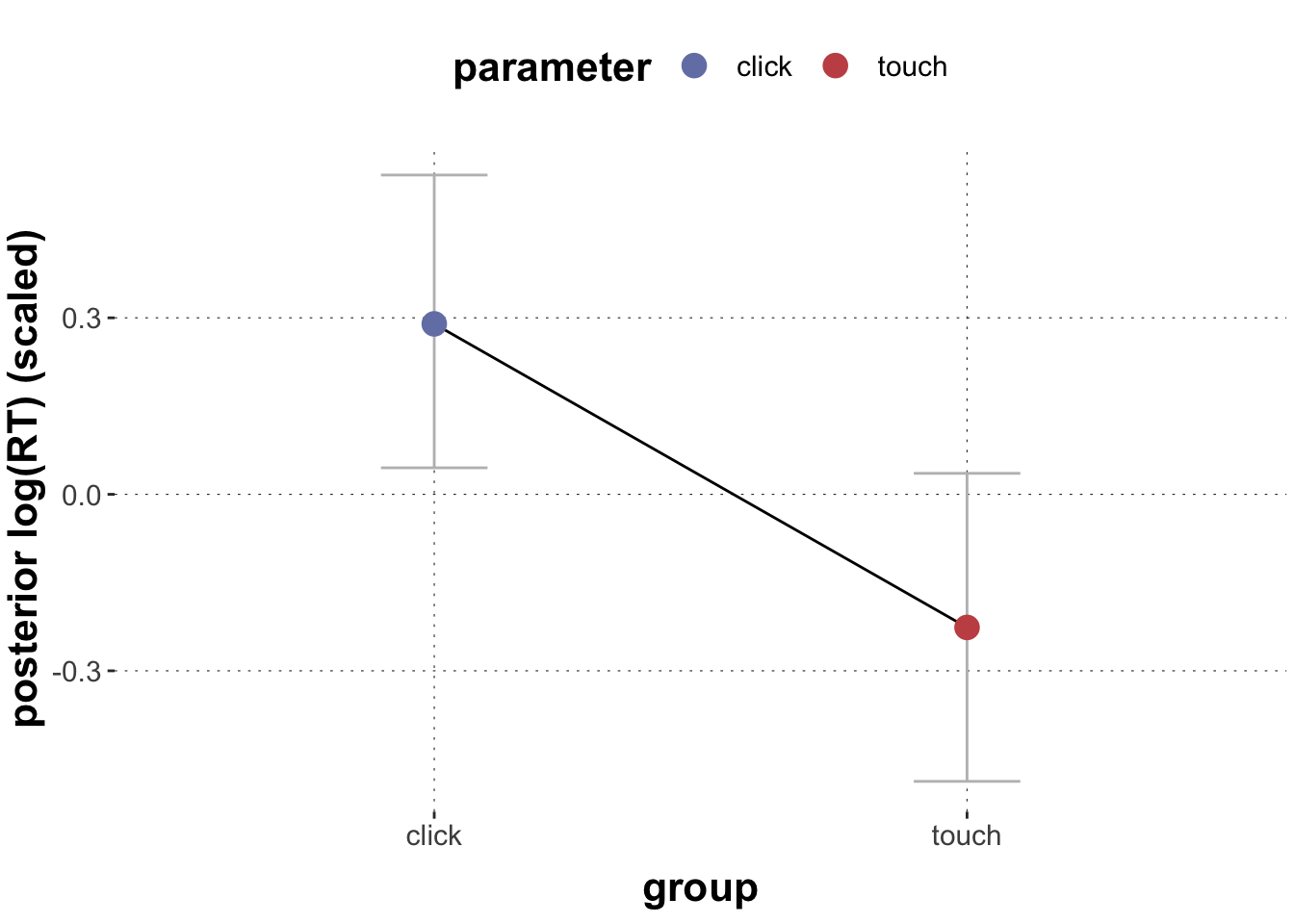
Intercept      0.29      0.13     0.04     0.54 1.01      465     1009
grouptouch    -0.52      0.12    -0.74    -0.28 1.01      447      937

Family Specific Parameters: 
      Estimate Est.Error l-95% CI u-95% CI Rhat Bulk_ESS Tail_ESS
sigma     0.68      0.01     0.66     0.71 1.00     5868     2566

Draws were sampled using sampling(NUTS). For each parameter, Bulk_ESS
and Tail_ESS are effective sample size measures, and Rhat is the potential
scale reduction factor on split chains (at convergence, Rhat = 1).

Exercise 1e

Extract the posterior means and 95% CrIs of touch vs. click log_RT_s and plot them.

Solution

Toggle code

# Extract the posteriors
posteriors <- xmdl %>%
  spread_draws(b_Intercept, 
               b_grouptouch) %>%
  # calculate posteriors for each individual level
  mutate(click = b_Intercept,
         touch = b_Intercept + b_grouptouch) %>% 
  select(click, touch) %>% 
  gather(key = "parameter", value = "posterior") %>% 
  group_by(parameter) %>% 
  summarise(mean_posterior = mean(posterior),
            `95lowerCrI` = HDInterval::hdi(posterior, credMass = 0.95)[1],
            `95higherCrI` = HDInterval::hdi(posterior, credMass = 0.95)[2])

# plot
ggplot(data = posteriors, 
       aes(x = parameter, y = mean_posterior,
           color = parameter, fill = parameter)) + 
  geom_errorbar(aes(ymin = `95lowerCrI`, ymax = `95higherCrI`),
                width = 0.2, color = "grey") +
  geom_line(aes(group = 1), color = "black") +
  geom_point(size = 4) +
  labs(x = "group",
       y = "posterior log(RT) (scaled)")

Exercise 1f

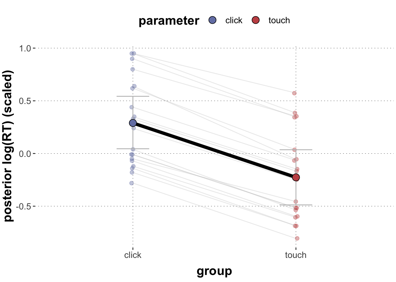
Add the posterior estimates for different exemplars to the plot. (Hint: Check code from the previous “tutorial” to extract the random effect estimates.)

Solution

Toggle code

# extract the random intercepts for exemplars
random_intc_matrix <- ranef(xmdl)$exemplar[, , "Intercept"] %>% 
  round(digits = 2) 

# extract the by-exemplar random slopes for group
random_slope_matrix <- ranef(xmdl)$exemplar[, , "grouptouch"] %>% 
  round(digits = 2)

# random intercepts to dataframe
random_intc_df <- data.frame(exemplar = row.names(random_intc_matrix), random_intc_matrix) %>% 
  select(exemplar, Estimate) %>% 
  rename(rintercept = Estimate)

# combine with random slope matrix
random_slope_df <- data.frame(exemplar = row.names(random_slope_matrix), random_slope_matrix) %>% 
  select(exemplar, Estimate) %>% 
  rename(rslope = Estimate) %>% 
  full_join(random_intc_df) %>% 
  # add population parameters and group-specific parameters
  mutate(click_population = fixef(xmdl)[1],
         touch_population = fixef(xmdl)[1] + fixef(xmdl)[2],
         click = rintercept + click_population,
         touch = rintercept + rslope + touch_population) %>% 
  select(exemplar, touch, click) %>% 
  gather(parameter, mean_posterior, -exemplar)
  

# combine with plot
ggplot(data = posteriors, 
       aes(x = parameter, y = mean_posterior,
           color = parameter, fill = parameter)) + 
   # add random estimates
  geom_point(data = random_slope_df, 
             alpha = 0.4,
             size = 2,
             position = position_jitter(width = 0.01)
             ) +
  # add lines between random estimates
  geom_line(data = random_slope_df, 
            aes(group = exemplar),
            color = "grey", alpha = 0.3) +
  # add population-level estimates
  geom_errorbar(aes(ymin = `95lowerCrI`, ymax = `95higherCrI`),
                width = 0.2, color = "grey") +
  geom_line(aes(group = 1), size = 2, color = "black") +
  geom_point(size = 4, pch = 21, color = "black") +
  labs(x = "group",
       y = "posterior log(RT) (scaled)")

Exercise 2: Poisson regression

Exercise 2a

Run a multilevel poisson regression predicting xpos_flips based on group, log_RT_s, and their two-way interaction. Specify maximal random effect structures for exemplars and subject_ids licensed by the design (ignore correlations between intercepts and slopes for now). (Hint: allow groupings to differ regarding the interaction effect if licensed by the design.) Specify weakly informative priors.

Solution

Toggle code

priors <- c(
  #priors for all fixed effects
  set_prior("student_t(3, 0, 3)", class = "b"),
  #prior for all SDs including the varying intercepts and slopes for both groupings
  set_prior("student_t(3, 0, 3)", class = "sd")
)

poisson_mdl <- brm(xpos_flips ~ group * log_RT_s +
                     (log_RT_s || subject_id) +
                     (group * log_RT_s || exemplar),
                   data = dolphin_correct,
                   prior = priors,
                   family = "poisson")

poisson_mdl

 Family: poisson 
  Links: mu = log 
Formula: xpos_flips ~ group * log_RT_s + (log_RT_s || subject_id) + (group * log_RT_s || exemplar) 
   Data: dolphin_correct (Number of observations: 1915) 
  Draws: 4 chains, each with iter = 2000; warmup = 1000; thin = 1;
         total post-warmup draws = 4000

Group-Level Effects: 
~exemplar (Number of levels: 19) 
                        Estimate Est.Error l-95% CI u-95% CI Rhat Bulk_ESS
sd(Intercept)               0.06      0.04     0.00     0.15 1.00     1473
sd(grouptouch)              0.11      0.07     0.00     0.26 1.00     1060
sd(log_RT_s)                0.04      0.04     0.00     0.13 1.00     1515
sd(grouptouch:log_RT_s)     0.08      0.06     0.00     0.22 1.00     1252
                        Tail_ESS
sd(Intercept)               1936
sd(grouptouch)              1842
sd(log_RT_s)                2086
sd(grouptouch:log_RT_s)     1861

~subject_id (Number of levels: 108) 
              Estimate Est.Error l-95% CI u-95% CI Rhat Bulk_ESS Tail_ESS
sd(Intercept)     0.59      0.06     0.49     0.71 1.00     1278     2285
sd(log_RT_s)      0.13      0.05     0.02     0.23 1.00      645      924

Population-Level Effects: 
                    Estimate Est.Error l-95% CI u-95% CI Rhat Bulk_ESS Tail_ESS
Intercept              -0.15      0.09    -0.33     0.03 1.00     1109     1665
grouptouch             -0.46      0.13    -0.72    -0.20 1.00     1379     1985
log_RT_s                0.39      0.05     0.30     0.49 1.00     2933     2994
grouptouch:log_RT_s     0.17      0.07     0.03     0.32 1.00     2769     2815

Draws were sampled using sampling(NUTS). For each parameter, Bulk_ESS
and Tail_ESS are effective sample size measures, and Rhat is the potential
scale reduction factor on split chains (at convergence, Rhat = 1).

Exercise 2b

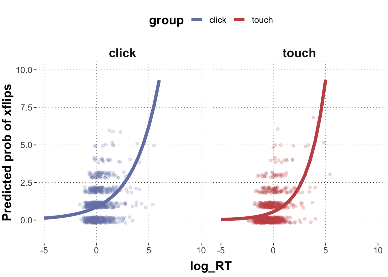
Extract and plot the population level estimates for both click and touch group as a regression line into a scatter plot (x = b_log_RT_s, y = xpos_flips).

Solution

Toggle code

# extract posterior means for model coefficients
predicted_Poisson_values <- poisson_mdl %>%
  spread_draws(b_Intercept, b_log_RT_s, 
               b_grouptouch, `b_grouptouch:log_RT_s`
               ) %>%
  # make a list of relevant value range of logRT
  mutate(log_RT = list(seq(-5, 10, 0.5))) %>% 
  unnest(log_RT) %>%
  mutate(click = exp(b_Intercept + b_log_RT_s*log_RT),
         touch = exp(b_Intercept + b_log_RT_s*log_RT +
                            b_grouptouch + `b_grouptouch:log_RT_s`*log_RT)) %>%
  select(log_RT, click, touch) %>% 
  gather(group, posterior, -log_RT) %>% 
  group_by(log_RT, group) %>%
  summarise(pred_m = mean(posterior, na.rm = TRUE),
            pred_low = quantile(posterior, prob = 0.025),
            pred_high = quantile(posterior, prob = 0.975)
            ) 

# plot population level
ggplot(data = predicted_Poisson_values, aes(x = log_RT, y = pred_m)) +
  geom_point(data = dolphin_correct, aes(x = log_RT_s, y = xpos_flips, color = group), 
             position = position_jitter(height = 0.2), alpha = 0.2) +
  geom_line(aes(y = pred_m, color = group), size = 2) +
  facet_grid(~group) +
  ylab("Predicted prob of xflips") +
  ylim(-1,10) +
  xlim(-5,10)

Exercise 2c

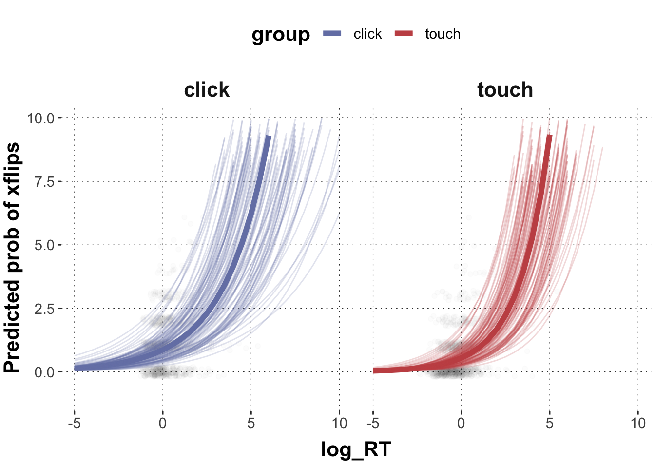
Extract the respective subject-specific estimates from the model and plot them into the same plot (use thinner lines).

Solution

Toggle code

# extract the random effects for subject_id

# intercepts
random_intc_matrix <- ranef(poisson_mdl)$subject_id[, , "Intercept"] %>% 
  round(digits = 3)

# slopes
random_slope_matrix <- ranef(poisson_mdl)$subject_id[, , "log_RT_s"] %>% 
  round(digits = 3)

# to df
random_intc_df <- data.frame(subject_id = row.names(random_intc_matrix), random_intc_matrix) %>% 
  select(subject_id, Estimate) %>% 
  rename(rintercept = Estimate)

# wrangle into one df 
random_slope_df <- data.frame(subject_id = row.names(random_slope_matrix), random_slope_matrix) %>% 
  select(subject_id, Estimate) %>% 
  rename(rslope = Estimate) %>% 
  full_join(random_intc_df) %>% 
  expand_grid(group = c("click", "touch")) %>% 
  # add population parameters and group-specific parameters
  mutate(adjusted_int = ifelse(group == "click",
           rintercept + fixef(poisson_mdl)[1],
           rintercept + fixef(poisson_mdl)[1] + fixef(poisson_mdl)[2]),
         adjusted_slope = ifelse(group == "click",
           rslope + fixef(poisson_mdl)[3],
           rslope + fixef(poisson_mdl)[3] + fixef(poisson_mdl)[4])) %>% 
  mutate(log_RT = list(seq(-5, 10, 0.5))) %>% 
  unnest(log_RT) %>%
  select(subject_id, log_RT, group, 
         adjusted_int, adjusted_slope) %>% 
  group_by(subject_id, log_RT, group) %>%
  mutate(pred_m = exp(adjusted_int + adjusted_slope*log_RT))

# plot the individual regression lines on top of the population estimate
ggplot(data = predicted_Poisson_values, aes(x = log_RT, y = pred_m)) +
  geom_point(data = dolphin_correct, aes(x = log_RT_s, y = xpos_flips), 
             position = position_jitter(height = 0.2), alpha = 0.01) +
  geom_line(aes(y = pred_m, color = group), size = 2) +
  geom_line(data = random_slope_df, 
            aes(x = log_RT, y = pred_m, group = subject_id, color = group),
            size = 0.5, alpha = 0.2) +
  facet_grid(~group) +
  ylab("Predicted prob of xflips") +
  ylim(-1,10) +
  xlim(-5,10)