Here is code to load (and if necessary, install) required packages, and to set some global options (for plotting and efficient fitting of Bayesian models).
Toggle code
# install packages from CRAN (unless installed)pckgs_needed <-c("tidyverse","brms","rstan","rstanarm","remotes","tidybayes","bridgesampling","shinystan","mgcv")pckgs_installed <-installed.packages()[,"Package"]pckgs_2_install <- pckgs_needed[!(pckgs_needed %in% pckgs_installed)]if(length(pckgs_2_install)) {install.packages(pckgs_2_install)} # install additional packages from GitHub (unless installed)if (!"aida"%in% pckgs_installed) { remotes::install_github("michael-franke/aida-package")}if (!"faintr"%in% pckgs_installed) { remotes::install_github("michael-franke/faintr")}if (!"cspplot"%in% pckgs_installed) { remotes::install_github("CogSciPrag/cspplot")}# load the required packagesx <-lapply(pckgs_needed, library, character.only =TRUE)library(aida)library(faintr)library(cspplot)# these options help Stan run fasteroptions(mc.cores = parallel::detectCores())# use the CSP-theme for plottingtheme_set(theme_csp())# global color scheme from CSPproject_colors = cspplot::list_colors() |>pull(hex)# names(project_colors) <- cspplot::list_colors() |> pull(name)# setting theme colors globallyscale_colour_discrete <-function(...) {scale_colour_manual(..., values = project_colors)}scale_fill_discrete <-function(...) {scale_fill_manual(..., values = project_colors)}
Simpson’s paradox: puzzle and data
Simpson’s paradox is a multi-faceted puzzle about how to analyse data, when the same data set can be interpreted differently, based on different assumptions about the causal relation between variables. The following uses a slight variation of a fictitious data set frequently used by Judea Pearl (e.g., in Pearl, Glymour and Jewell (“Causal Inference in Statistics: A primer”, 2016)). There are two scenarios, to be introduced one after the other below, framed as data about the effect of a drug on the rate of recovery.
The most important objective of this tutorial is to calculate the total causal effect (TCE) of the drug in each scenario, following the approach outlined by Pearl et al. (2016). We first calculate a maximum-likelihood estimate of the TCE and then a Bayesian estimate derived from regression modeling. The advantage of the latter is that it allows quantification of uncertainty of the TCE estimate.
Case 1: Gender
In the first scenario (referred to as “Case 1: Gender as a confound”), the data was collected by the following procedure:
700 participants were recruited, out of which 357 identified as male and 343 identified as female
each participant decided whether or not to take the drug
we observed whether the participant recovered or not (binary outcome)
Here is the data for the first scenario:
Toggle code
################################################### set up the data for SP##################################################data_simpsons_paradox <-tibble(gender =c("Male", "Male", "Female", "Female"),bloodP =c("Low", "Low", "High", "High"),drug =c("Take", "Refuse", "Take", "Refuse"),k =c(81, 234, 192, 55),N =c(87, 270, 263, 80),proportion = k/N)data_simpsons_paradox |>select(-bloodP)
# A tibble: 4 × 5
  gender drug       k     N proportion
  <chr>  <chr>  <dbl> <dbl>      <dbl>
1 Male   Take      81    87      0.931
2 Male   Refuse   234   270      0.867
3 Female Take     192   263      0.730
4 Female Refuse    55    80      0.688
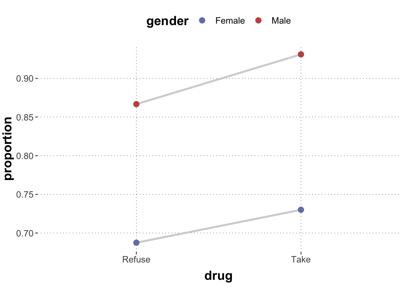
Research Team 1 bends over this data set and notices that the drug increases recovery for both males and females, as shown in the plot below. Based on this, Research Team 1 concludes that the drug is effective and they recommend its usage.
Toggle code
data_simpsons_paradox |>ggplot(aes(x = drug, y = proportion, group = gender)) +geom_line(size =1.2, color = project_colors[12]) +geom_point(size =3, aes(color = gender))
Case 2: Blood pressure
But now consider a second scenario. Data was collected by the following process:
700 participants were recruited
each participant decided whether or not to take the drug
each participant’s blood pressure is measured and, based on this measurement, the participant is assigned to a high and low blood pressure group (measurement happens after having taken the drug)
we observed whether each participant recovered or not
The data for this scenario look as follows:
Toggle code
data_simpsons_paradox |>select(-gender)
# A tibble: 4 × 5
  bloodP drug       k     N proportion
  <chr>  <chr>  <dbl> <dbl>      <dbl>
1 Low    Take      81    87      0.931
2 Low    Refuse   234   270      0.867
3 High   Take     192   263      0.730
4 High   Refuse    55    80      0.688
(Yes, you are right! The numbers are exactly the same as before!)
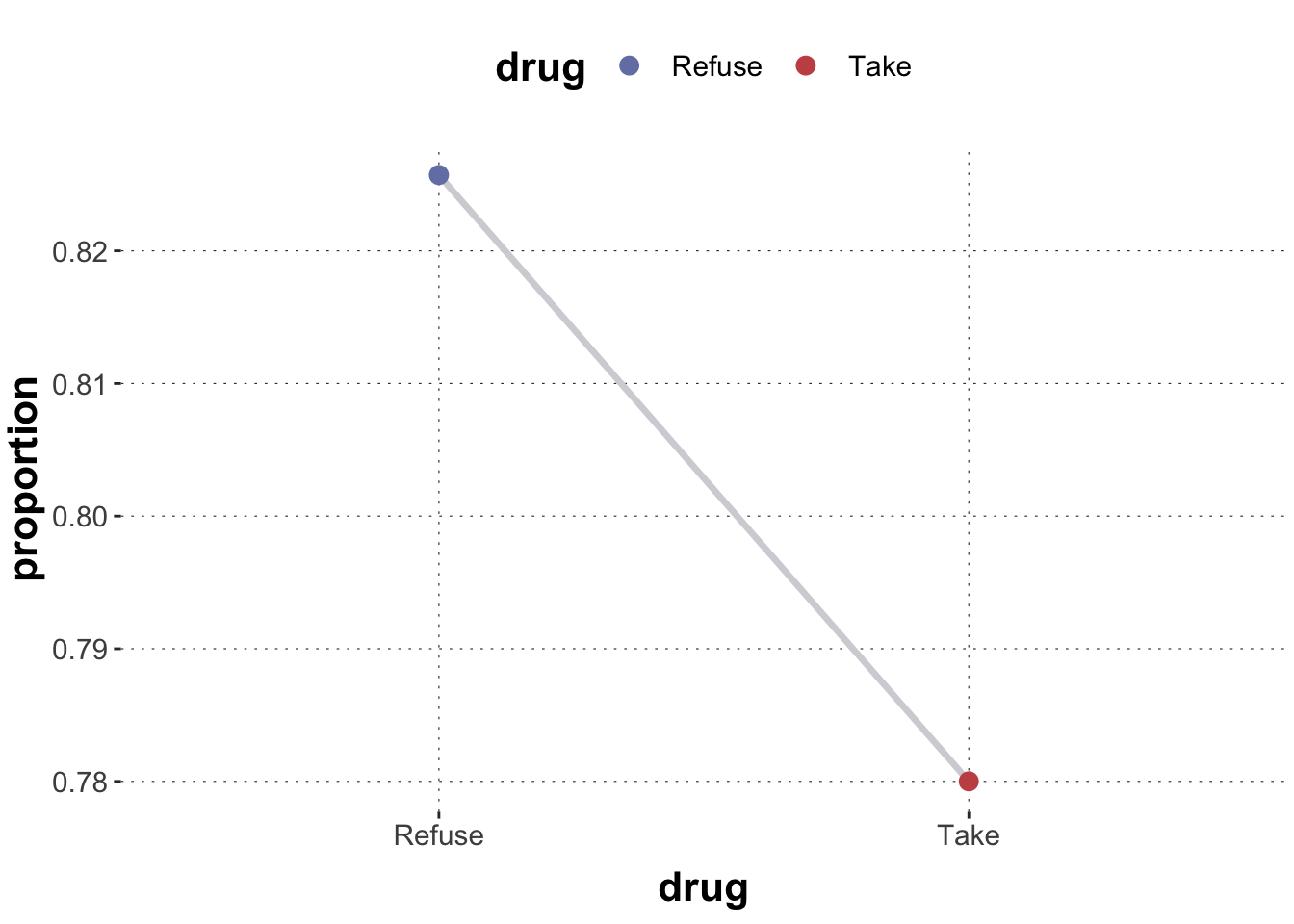
Research Team 2 bends over this data set and notices that the drug decreases recovery rate in the whole population, as shown in the plot below. Based on this, Research Team 2 concludes that the drug is not effective. They do not recommend it for usage.
The puzzle here is that two research teams have reached opposite conclusions based on data which is at least numerically the exact same. Each team seems, at first glance, to have drawn reasonable conclusions. How is it possible to reach opposite conclusions about whether or not to use a drug, based on the same set of numbers?
Resolving the puzzle by causal analysis
You say: “The data sets are not the same! The numbers are, but in one case we observed gender and in the other we observed blood pressure. That makes a difference, doesn’t it?”
I say: “Well, okay, but not necessarily. Just having different labels for levels of a categorical variable doesn’t make for a different data set, does it?”
But you immediately shoot back: “Maybe, but you also told us about a difference in the data-generating process. There is at least a temporal difference: blood pressure is measured after the treatment, but the level of gender was fixed already before the treatment.”
“Okay” I say. “So, do you suggest a temporal analysis?”
You roll your eyes and after a few more (ridiculous) turns of this conversation, we both agree that, at least conceptually speaking, there is a difference in the plausible causal structure of the involved variables.
Consider the first case. There are three binary variables involved. Given the temporal sequence of events in the data-generating process, the likely causal relation between the variables is that gender may influence both drug (the decision to take the drug or not) and recovery. Moreover, the drug may have influenced recovery directly.
Causal structure of scenario 1: gender is a confound
Now consider the second scenario. Again, we have three binary variables. But since blood pressure is measured after the treatment, it is not plausible that it could have influenced the decision of whether to take the drug or not. Reversely, it is plausible to assume, i.e., to at least allow for the possibility, that blood pressure was affected by gender and that it may have affected recovery. As before, we also make room for the possibility that drug may affect recovery also directly.
Causal structure of scenario 2: blood pressure is a mediator
Causal analysis with MLE
Following Pearl’s approach to causal analysis, the most important quantity to assess is how (hypothetical) manipulations of administering the drug would influence the recovery rate. In other words, we would like to quantify the total causal effect (TCE):
as the difference in expected recovery rate in the imagined scenario that we could surgically change whether a drug was given, without changing non-causal dependencies of drug.
What it means to condition on “\(\mathit{do}(D=d)\)” depends on the assumed causal relationship between variables. So, we will look at each scenario in sequence.
Case 1: Gender as a confound
Since the set \(\{G\}\) statisfies the backdoor criterion for the assumed causal DAG, we know that we can calculate the total causal effect (TCE) by eliminating the do-operator in the conditioning using the adjustment formula:
This means that we need to estimate two probability distributions: the conditional probability of recovery given drug and gender and the (marginal) probability of gender. We can use maximum-likelihood estimates for these by just using the observed frequencies as estimators. For \(\mathit{do}(D=1)\), this yields:
This suggest that the drug is effectively increasing expected recovery, but we do not have a measure of uncertainty of this estimate. We don’t know if we should consider this convincing evidence to recommend wide-spread adoption. That’s why we need (something like) Bayesian estimation eventually. But let’s first look at the second scenario.
Case 2: Blood pressure as a mediator
For the causal graph assumed for the second scenario, the do-intervention reduces to the conditional probability:
This differs in sign from the previous estimate, and we might conclude that administering the drug is, overall, not beneficial. Yet, again, we have no uncertainty quantification regarding this estimate.
Bayesian causal effect estimation
Let’s use Bayesian regression modelling to calculate the total causal effects for each scenario.
Some data wrangling
For subsequent analysis (especially when generating predictive samples), it helps to have the data in long format. The uncount() function is a great tool for this.
Toggle code
# cast into long formatdata_SP_long <-rbind( data_simpsons_paradox |>uncount(k) |>mutate(recover =TRUE) |>select(-N, -proportion), data_simpsons_paradox |>uncount(N-k) |>mutate(recover =FALSE) |>select(-N, -proportion, -k))data_SP_long
# A tibble: 700 × 4
   gender bloodP drug  recover
   <chr>  <chr>  <chr> <lgl>
 1 Male   Low    Take  TRUE
 2 Male   Low    Take  TRUE
 3 Male   Low    Take  TRUE
 4 Male   Low    Take  TRUE
 5 Male   Low    Take  TRUE
 6 Male   Low    Take  TRUE
 7 Male   Low    Take  TRUE
 8 Male   Low    Take  TRUE
 9 Male   Low    Take  TRUE
10 Male   Low    Take  TRUE
# ℹ 690 more rows
Case 1: Gender as a confound
Given the causal structure assumed for scenario 1, we can calculate the effects of the relevant do-intervention as:
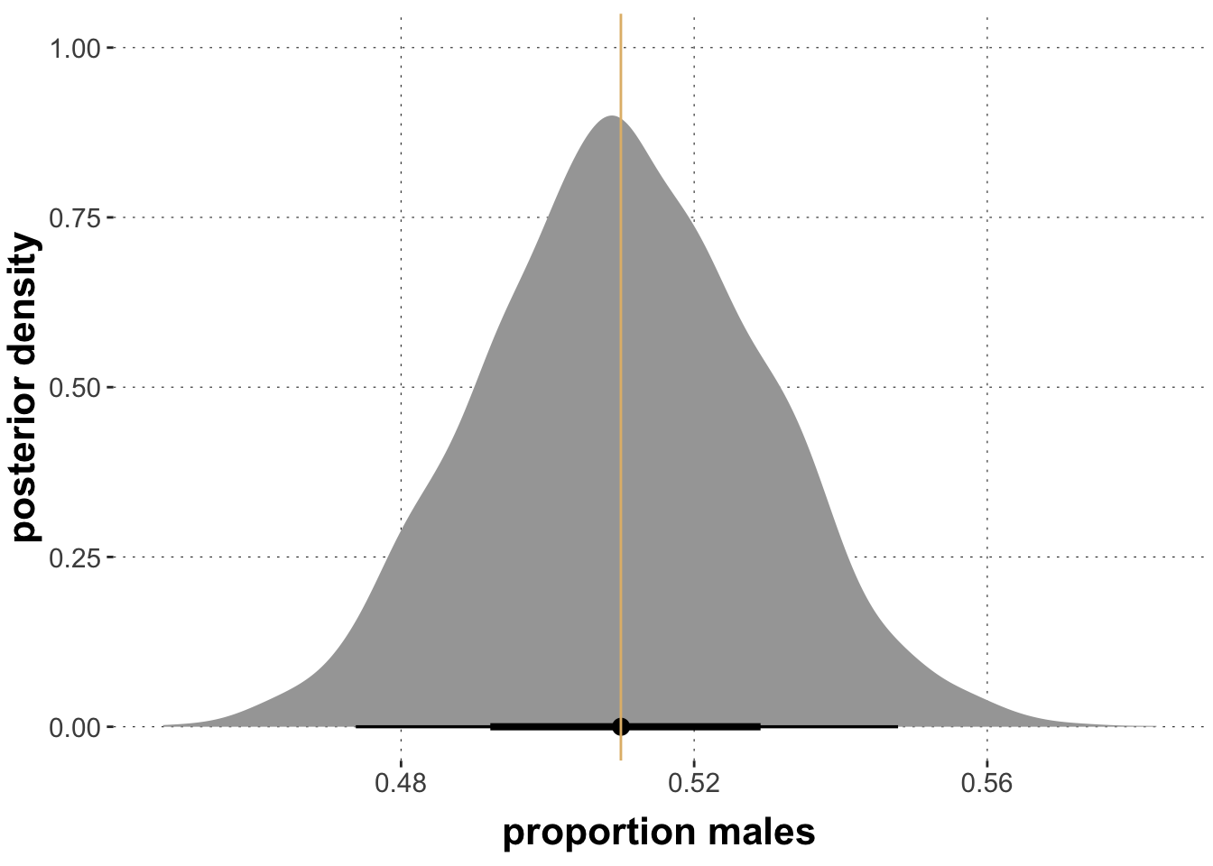
Each sample from the posterior of the Intercept parameter represents (a guess of) the log-odds of the Male category. The posterior over the proportion of male participants can therefore be retrieved and plotted as follows (the yellow line shows the observed frequency):
Step 3: Compute the posterior expectations and the TCE
In a third step, we draw posterior predictive samples for the model from step 2, based on posterior predictive samples for the model from step 1, while manually setting drug to Take and Refuse.
First, we get posterior predictive samples of gender from the model from step 1. Notice that these are just samples of Male and Female, for which we will generate predictions based on the the second model.
Toggle code
postPred_gender <- tidybayes::predicted_draws(object = fit_SP_GonIntercept,newdata =tibble(Intercept =1),value ="gender",ndraws = niter *2 ) |>ungroup() |>mutate(gender =ifelse(gender, "Male", "Female")) |>select(gender)# NB: in this case we could also have gotten this via: # rbinom(n=4000, p=rbeta(4000, 315+1, 700-315+1), size = 700)postPred_gender
Based on these ‘sampled individuals’ we generate the prediction of the second model (predicting the a posteriori expected recovery, given gender and whether to take the drug or not).
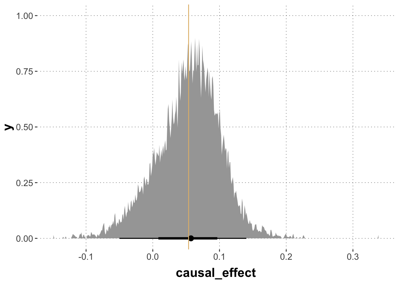
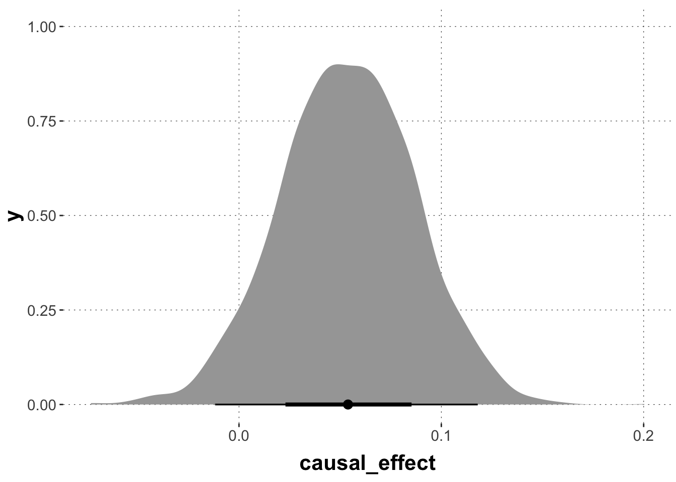
This yields a point estimate (Bayesian mean posterior) and the usual uncertainty quantification in terms of credible intervals etc. In this case, we would not be compelled to conclude that the causal effect is substantial as the posterior estimate for this effect clearly encompasses non-negligible mass for the range of negative values. The orange line show the maximum-likelihood estimate of the causal effect.
Exercise 1: Alternative calculation of causal effect estimate
The last plot looks a bit ragged. This is because we approximate \(P(G)\) by actual samples of levels Male and Female. There is an alternative, though. Both approaches are correct. But they differ slightly in logic and execution, so you may benefit from having seen both.
In this new approach you do this:
Approximate \(P(G)\) by taking samples from the expected value of \(P(G=M)\). Use the function tidybayes::epred_draws() for this.
Sample expected values of \(P(R=1 \mid G, D)\) for all combinations of levels of \(G\) and \(D\).
Weigh the predicted recovery rates from step 2 with the corresponding predictions of \(P(G)\) from step 1.
Compute the causal effect from this.
Compute the ususal summary statistics (posterior mean, credible interval) and plot the posterior for the estimated causal effect.
Solution
Toggle code
# get epred samples for intercept-only model:postPred_maleProportion <- tidybayes::epred_draws( fit_SP_GonIntercept, newdata =tibble(Intercept =1),value ="maleProp",ndraws = niter *2 ) |>ungroup() |>select(.draw, maleProp)# get epred samples for the R ~ D, G model# for all combinations of D and Gposterior_DrugTaken <- tidybayes::epred_draws(object = fit_SP_RonGD,newdata =tibble(gender =c("Male", "Male", "Female", "Female"),drug =c("Take", "Refuse", "Take", "Refuse")),value ="recovery",ndraws = niter *2) |>ungroup() |>select(.draw, gender, drug, recovery)# weigh and compute the causal effectCE_post <- posterior_DrugTaken |>full_join( postPred_maleProportion) |>mutate(weights =ifelse(gender =="Male", maleProp, 1-maleProp)) |>group_by(`.draw`, drug) |>summarize(predRecover =sum(recovery * weights)) |>pivot_wider(names_from = drug, values_from = predRecover) |>mutate(causal_effect = Take - Refuse) # produce summary statisticsrbind( aida::summarize_sample_vector(CE_post$Take, "drug_taken"), aida::summarize_sample_vector(CE_post$Refuse, "drug_refused"), aida::summarize_sample_vector(CE_post$causal_effect, "causal_effect"))
# plot the relevant posteriorCE_post |>ggplot(aes(x = causal_effect)) + tidybayes::stat_halfeye()
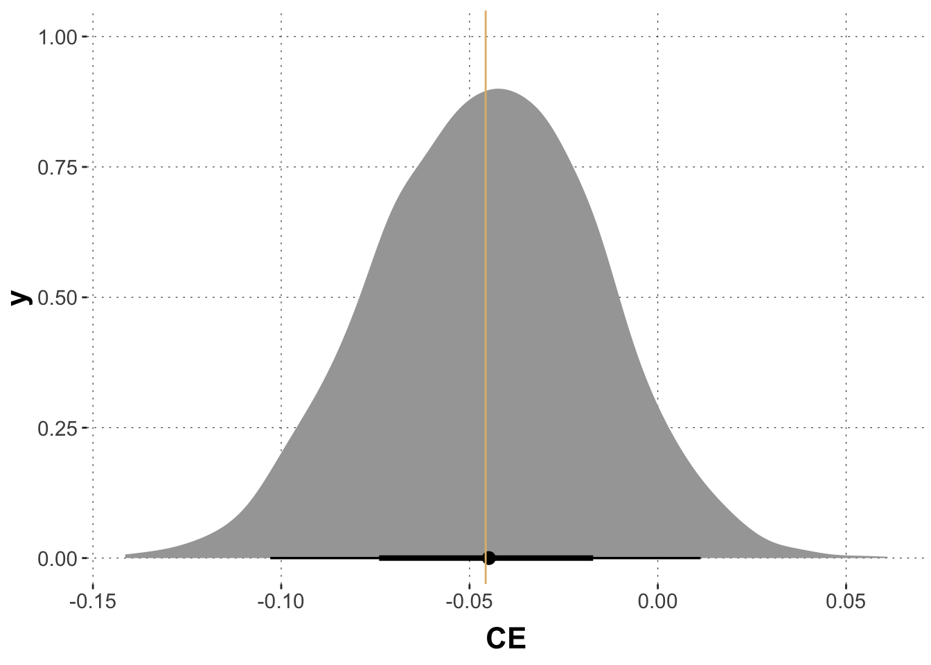
Case 2: Blood pressure as a mediator
For the second case, blood pressure as a mediator, the calculations are much easier. We just need to estimate \(P(R \mid D, B)\), so a single regression model will do.
The coefficients of a logistic regression model relate to log-odds. Using the faintr package and the logistic transformation, we can calculate samples of the causal effect as follows:
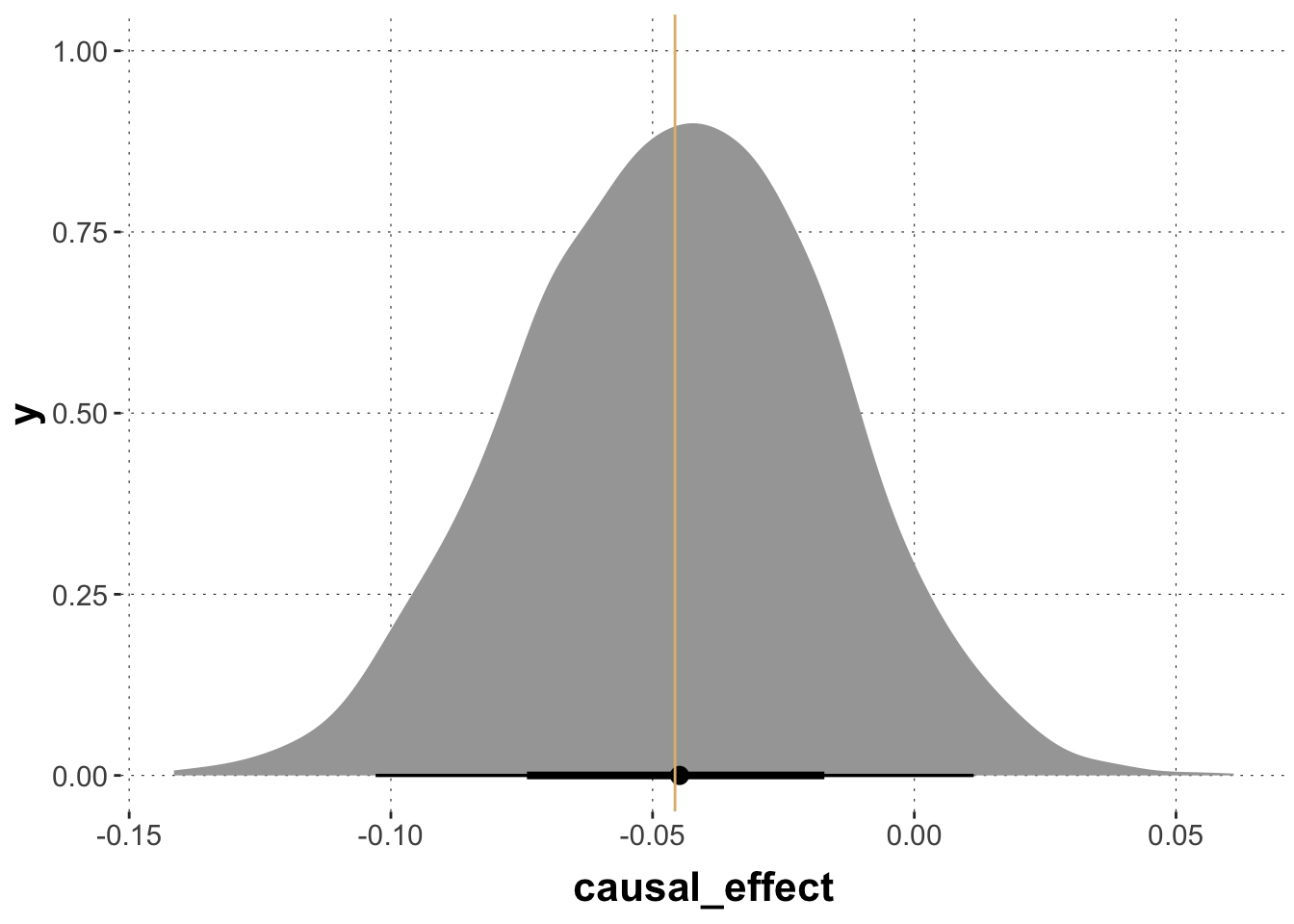
Exercise 2: Using poterior predictives to estimate causal effects
The last section computed estimates of the relevant causal effect directly from the samples for model coefficients. This works well for logistic regression, but in other cases it may be more convenient to use samples from the posterior predictive distribution of the R ~ D, G model, similar to what we did in the first scenario.
So, use tidybayes::epred_draws() to get estimates of the causal effect.