XX: Distributional models

Bayesian regression: theory & practice

The term “distributional model” is not sharply defined and not altogether common. Alternatively, one may read “models for location, scale and shape” or similar verbiage. The general idea, however, is simple: when our model has a likelihood function with additional parameters, e.g., the standard deviation \(\sigma\) in the Gaussian likelihood function of a vanilla linear regression, we can not only infer these parameters, but also make them dependent, e.g., on other predictors.

For example, when a standard linear regression model would look like this:

\[ \begin{align*} y & \sim \mathcal{N}(\mu, \sigma) \\ \mu & = X \ \beta \\ \beta, \sigma & \sim \dots \text{some priors} \dots \end{align*} \]

a simple distributional model could look like this:

\[ \begin{align*} y & \sim \mathcal{N}(\mu, \sigma) \\ \mu & = X \ \beta^{\mu} \\ \sigma & = \exp \left ( X \ \beta^{\sigma} \right) \\ \beta^{\mu}, \beta^{\sigma} & \sim \dots \text{some priors} \dots \end{align*} \]

thereby assuming that \(\sigma\) itself depends on the predictors \(X\) in a linear way.

Preamble

Here is code to load (and if necessary, install) required packages, and to set some global options (for plotting and efficient fitting of Bayesian models).

Toggle code

# install packages from CRAN (unless installed)
pckgs_needed <- c(
  "tidyverse",
  "brms",
  "rstan",
  "rstanarm",
  "remotes",
  "tidybayes",
  "bridgesampling",
  "shinystan",
  "mgcv"
)
pckgs_installed <- installed.packages()[,"Package"]
pckgs_2_install <- pckgs_needed[!(pckgs_needed %in% pckgs_installed)]
if(length(pckgs_2_install)) {
  install.packages(pckgs_2_install)
} 

# install additional packages from GitHub (unless installed)
if (! "aida" %in% pckgs_installed) {
  remotes::install_github("michael-franke/aida-package")
}
if (! "faintr" %in% pckgs_installed) {
  remotes::install_github("michael-franke/faintr")
}
if (! "cspplot" %in% pckgs_installed) {
  remotes::install_github("CogSciPrag/cspplot")
}

# load the required packages
x <- lapply(pckgs_needed, library, character.only = TRUE)
library(aida)
library(faintr)
library(cspplot)

# these options help Stan run faster
options(mc.cores = parallel::detectCores())

# use the CSP-theme for plotting
theme_set(theme_csp())

# global color scheme from CSP
project_colors = cspplot::list_colors() |> pull(hex)
# names(project_colors) <- cspplot::list_colors() |> pull(name)

# setting theme colors globally
scale_colour_discrete <- function(...) {
  scale_colour_manual(..., values = project_colors)
}
scale_fill_discrete <- function(...) {
   scale_fill_manual(..., values = project_colors)
}

Example: World temperature data

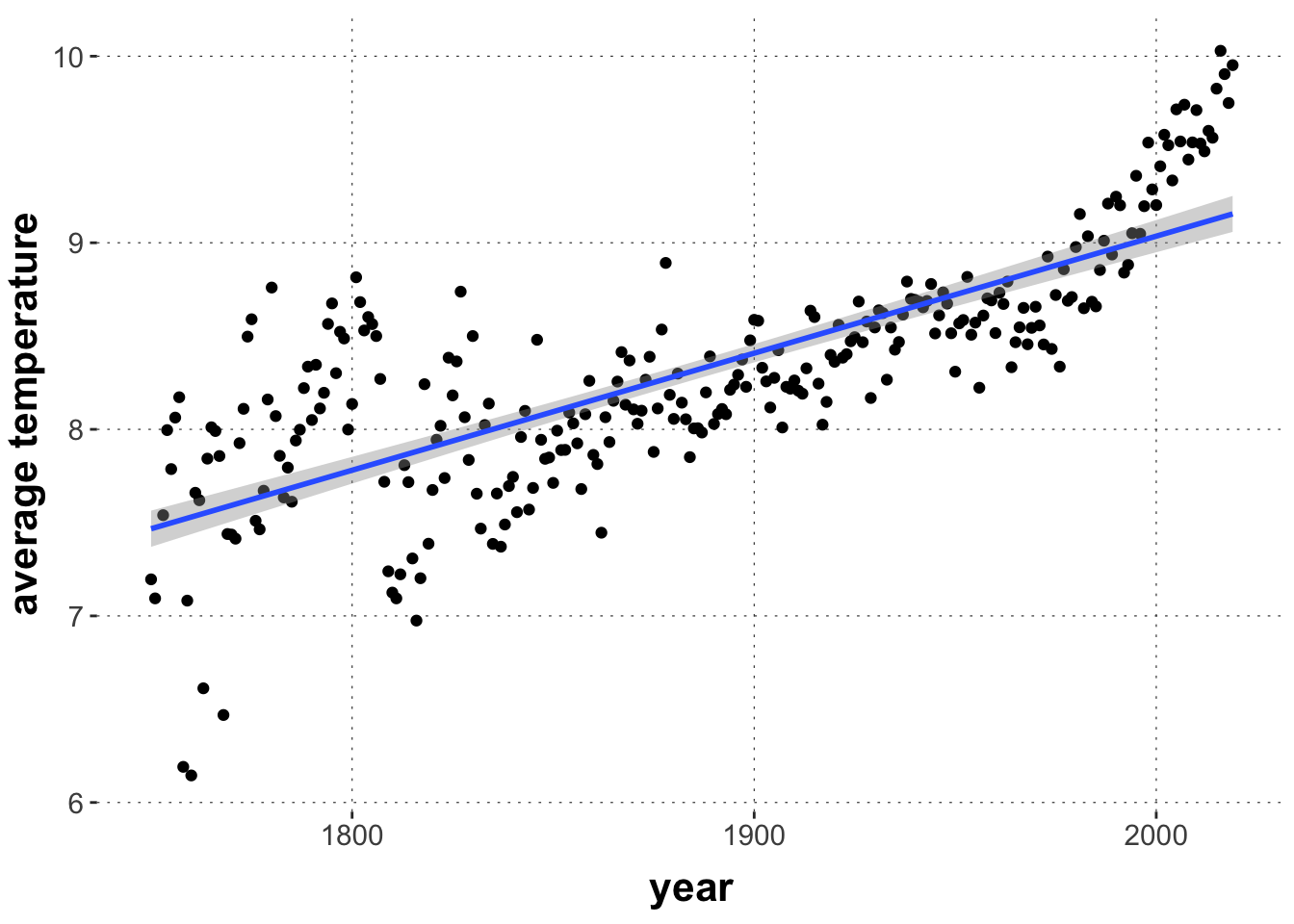
The World Temperature data, included in the aida package provides a useful minimal example. We want to regress avg_temp on year, but we see that early measurements appear to be much more noisy, so that a linear fit will be better for data between 1900 and 1980, and worse for data between 1750 to 1900, simply because of differences related to differently noise measurements at different times.

Toggle code

aida::data_WorldTemp |> 
  ggplot(aes(x = year, y = avg_temp)) +
  geom_point() +
  ylab("average temperature") + geom_smooth(method = "lm")

A simple linear regression model is easy to fit:

Toggle code

# vanilla regression
fit_temp_vanilla <- 
  brms::brm(
    avg_temp ~ year,
    data = aida::data_WorldTemp)

But there are clear indicators that this is not a very good model, e.g., using a posterior predictive \(p\)-value with the standard deviation for predictions of all data points between 1750-1800 as a test statistic:

Toggle code

postPred_y <- 
  tidybayes::predicted_draws(
    object  = fit_temp_vanilla,
    newdata = aida::data_WorldTemp |> dplyr::select(year) |> filter(year <= 1800),
    value   = "avg_temp",
    ndraws  = 4000) |> ungroup() |> 
  dplyr::select(.draw, year, avg_temp)

sd_postPred <- postPred_y |> 
  group_by(.draw) |> 
  summarize(sd_post_pred = sd(avg_temp)) |> 
  pull(sd_post_pred)

sd_data <- aida::data_WorldTemp |> filter(year <= 1800) |> pull(avg_temp) |> sd()

mean(sd_data > sd_postPred)

[1] 1

If we care about faithful prediction in this early period, including accuracy about the noisiness of the data, the vanilla linear model is clearly bad.

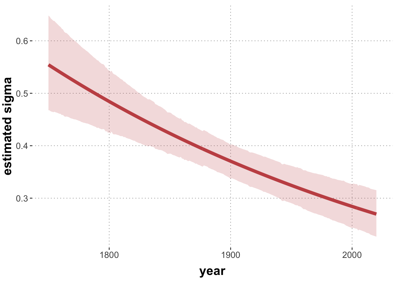
A simple distributional model

We want to fit the distributional model sketched in the beginning:

\[ \begin{align*} y & \sim \mathcal{N}(\mu, \sigma) \\ \mu & = X \ \beta^{\mu} \\ \sigma & = \exp \left ( X \ \beta^{\sigma} \right) \\ \beta^{\mu}, \beta^{\sigma} & \sim \dots \text{some priors} \dots \end{align*} \]

To fit this model with brms, we need to specify the formula for the regression as follows:

Toggle code

formula_temp_distributional = brms::bf(avg_temp ~ year, sigma ~ year)

This formula first declares that avg_temp is to be regressed on year, as usual, and also declares that sigma is supposed to be regressed (in quite the same way) on year as well. The variable sigma does not occur in the data, but is recognized as an internal variable, namely the standard deviation of the Gaussian likelihood function.

Sampling with Stan can get troublesome if parameters are on quite different scales, so we should make sure that the two estimands are roughly on the same scale.

Toggle code

# to run a distributional model, we need to rescale 'year'
#   division by a factor of 1000 is sufficient
data_WorldTemp <- aida::data_WorldTemp |> 
  mutate(year = (year)/1000)

Toggle code

fit_temp_distributional <- 
  brms::brm( 
    formula = brms::bf(avg_temp ~ year, sigma ~ year),
    data    = data_WorldTemp
  )

This model provides us with information about intercepts and slopes for both components, the regression of avg_temp and sigma.

Toggle code

summary(fit_temp_distributional)

 Family: gaussian 
  Links: mu = identity; sigma = log 
Formula: avg_temp ~ year 
         sigma ~ year
   Data: data_WorldTemp (Number of observations: 269) 
  Draws: 4 chains, each with iter = 2000; warmup = 1000; thin = 1;
         total post-warmup draws = 4000

Population-Level Effects: 
                Estimate Est.Error l-95% CI u-95% CI Rhat Bulk_ESS Tail_ESS
Intercept          -5.07      0.67    -6.42    -3.79 1.00     3149     2915
sigma_Intercept     4.08      1.00     2.12     6.06 1.00     2929     2745
year                7.09      0.35     6.42     7.79 1.00     3191     2938
sigma_year         -2.67      0.53    -3.71    -1.64 1.00     2916     2728

Draws were sampled using sampling(NUTS). For each parameter, Bulk_ESS
and Tail_ESS are effective sample size measures, and Rhat is the potential
scale reduction factor on split chains (at convergence, Rhat = 1).

Here is a plot that shows the posterior (means and credible interval) of \(\sigma\) as a function of year.

Toggle code

tidybayes::tidy_draws(fit_temp_distributional) |> 
  dplyr::select(.draw, b_sigma_Intercept, b_sigma_year) |> 
  cross_join(tibble(year = (1750:2020) / 1000)) |>
  mutate(sigma_predicted = exp(b_sigma_Intercept + b_sigma_year * year)) |> 
  group_by(year) |> 
  summarize(
    lower  = tidybayes::hdi(sigma_predicted)[1],
    mean   = mean(sigma_predicted),
    higher = tidybayes::hdi(sigma_predicted)[2]) |> 
  ggplot(aes(x = year * 1000, y = mean)) +
  geom_ribbon(aes(ymin=lower, ymax=higher), fill = project_colors[2], alpha = 0.2) +
  geom_line(color = project_colors[2], linewidth = 2) +
  xlab("year") +
  ylab("estimated sigma")

Exercise 1a

Let’s inspect how brms sets up the priors for this model:

Toggle code

brms::get_prior(
  formula = brms::bf(avg_temp ~ year, sigma ~ year),
  data    = data_WorldTemp)

                  prior     class coef group resp  dpar nlpar lb ub
 student_t(3, 8.3, 2.5) Intercept                                  
                 (flat)         b                                  
                 (flat)         b year                             
   student_t(3, 0, 2.5) Intercept                 sigma            
                 (flat)         b                 sigma            
                 (flat)         b year            sigma            
       source
      default
      default
 (vectorized)
      default
      default
 (vectorized)

Using this information set a prior on the slope coefficient for both components of the model. Use a Student-t distribution with one degree of freedom, mean 0 and standard deviation 10.

Solution

Toggle code

prior_temp_distributional <- 
  c(prior(student_t(1,0,10), class = "b", coef = "year_c"),
    prior(student_t(1,0,10), class = "b", dpar = "sigma")
    )