Gaussian process regression in `brms`

Bayesian regression: theory & practice

Author

Michael Franke

This tutorial provides both a brief conceptual introduction into Gaussian process regression. It develops intuitions about how, from a generalization of multi-variate normal distributions, we can obtain something like a “prior over functions”. It also demonstrates how a Gaussian process regression can be implemented in brms.

Preamble

Here is code to load (and if necessary, install) required packages, and to set some global options (for plotting and efficient fitting of Bayesian models).

Toggle code

# install packages from CRAN (unless installed)
pckgs_needed <- c(
  "tidyverse",
  "brms",
  "rstan",
  "rstanarm",
  "remotes",
  "tidybayes",
  "bridgesampling",
  "shinystan",
  "mgcv"
)
pckgs_installed <- installed.packages()[,"Package"]
pckgs_2_install <- pckgs_needed[!(pckgs_needed %in% pckgs_installed)]
if(length(pckgs_2_install)) {
  install.packages(pckgs_2_install)
} 

# install additional packages from GitHub (unless installed)
if (! "aida" %in% pckgs_installed) {
  remotes::install_github("michael-franke/aida-package")
}
if (! "faintr" %in% pckgs_installed) {
  remotes::install_github("michael-franke/faintr")
}
if (! "cspplot" %in% pckgs_installed) {
  remotes::install_github("CogSciPrag/cspplot")
}

# load the required packages
x <- lapply(pckgs_needed, library, character.only = TRUE)
library(aida)
library(faintr)
library(cspplot)

# these options help Stan run faster
options(mc.cores = parallel::detectCores())

# use the CSP-theme for plotting
theme_set(theme_csp())

# global color scheme from CSP
project_colors = cspplot::list_colors() |> pull(hex)
# names(project_colors) <- cspplot::list_colors() |> pull(name)

# setting theme colors globally
scale_colour_discrete <- function(...) {
  scale_colour_manual(..., values = project_colors)
}
scale_fill_discrete <- function(...) {
   scale_fill_manual(..., values = project_colors)
}

Gaussian processes

A Gaussian process is a generalization of a multi-variate normal distribution, which in turn is a generalization of a simple normal distribution. A simple normal distribution provides a likelihood for a single response variable \(y\) based on a pair of single numbers for mean \(x\) and standard deviation \(\sigma\):

\[ y \sim \mathcal{N}(x, \sigma) \]

A multivariate Gaussian extends this to provide a probability of a vector \(\mathbf{y}\) of \(k\) finite numbers for a \(k\)-place vector of means \(\mathbf{x}\) and a \(k \times k\) covariance matrix \(\Sigma\):

\[ \mathbf{y} \sim \text{MV-Normal}(\mathbf{x}, \Sigma) \]

One heuristic way of thinking of a Gaussian process is as a whole (infinite) set of systematically related multi-variate normal distributions. For each vector \(\mathbf{x}\) of means, with arbitrary finite length \(k\), this set contains a multi-variate normal distribution for us. So, we are not stuck with one specific \(k\), but we have exactly one for each \(\mathbf{x}\) no matter what \(k\), as long as it is finite.

To obtain such a set, we construct a function which, for a given \(\mathbf{x}\), constructs a covariance matrix \(\Sigma\) for us in a systematic way. This is done via a so-called kernel. The kernel is what gives us the “systematicity” in our set of multi-variate normal distributions. (It also regulates the overal shape of functions implied by the Gaussian process; more on this below.)

There are many different useful kernels, but the most salient one is perhaps the radial basis function kernel. It is defined as follows:

\[ k(\mathbf{x},\mathbf{x}') = \sigma_f^2 \ \exp \left [ - \frac{||\mathbf{x} - \mathbf{x}'||^2}{2 \lambda}\right] \]

Here \(||\cdot||\) is the Euclidean norm, defined as \(||\mathbf{x}|| = \sqrt{x_1^2 + \dots + x_k^2}\), an expression of the length of a vector. There are two parameters in the radial basis kernel:

\(\sigma_f\) is signal variance, and
\(\lambda\) is the *length scale.

For a given vector \(\mathbf{x}\), we can use the kernel to construct finite multi-variate normal distribution associated with it like so:

\[ \mathbf{x} \mapsto_{GP} \text{MV-Norm}(m(\mathbf{x}), k(\mathbf{x}, \mathbf{x})) \]

where \(m\) is a function that specifies the mean for the distribution associated with \(\mathbf{x}\). This mapping is essentially the Gaussian process: a systematic association of vectors of arbitrary length with a suitable multi-variate normal distribution.

A compact prior over functions

Cool, but why do we care? We care because a Gaussian process (GP) allows us to specify a vast amount of non-linear curves, so to speak. More concretely, a GP, defined by a kernel \(k(\cdot)\), a mean function \(m(\cdot)\), and the parameters \(\sigma_f\) and \(\lambda\), implies a prior of functions. This is very abstract and best explored through simulation.

Here are two convenience functions. The first is called get_GP_simulation and it samples from a Gaussian process regression. It takes as input a vector x to generated predictions for, values for the kernel parameters sigma_f and lambda and also the usual simple linear regression parameters Intercept, slope and sigma. The second function is called plot_GP_simulation takes as input what the first function delivers and provides a plot.

Using these functions we can explore how we can “generate wiggly lines” for different input vectors x and parameter settings.

Toggle code

get_GP_simulation <- 
  function(x = seq(0,10, by = 0.1), 
           Intercept = 0, 
           slope = 1, 
           sigma = 1, 
           sigma_f=0.5, 
           lambda=100, 
           seed = NULL) {
    
    if (! is.null(seed)){
      set.seed(seed)
    }
    
    # number of points to generate prediction for
    N <- length(x)
    
    # linear predictor (vanilla LM)
    eta = Intercept + slope * x
    
    # kernel function (here: radial basis function kernel)
    get_covmatrix <- function(x, sigma_f, lambda) {
      K = matrix(0, nrow=N, ncol=N)
      for (i in 1:N) {
        for (j in 1:N) {
          K[i,j] = sigma_f^2 * exp(sqrt((i-j)^2) / (-2 *lambda))
        }
      }
      return(K)
    }
    
    # covariance matrix
    K <- get_covmatrix(x, sigma_f, lambda)
    
    # Gaussian process wiggles
    epsilon_gp <- mvtnorm::rmvnorm(
      n     = 1, 
      mean  = rep(0, N),
      sigma = K)[1,]
    
    # central tendency
    mu <- epsilon_gp + eta
    
    # data prediction
    y <- rnorm(N, mu, sigma)
      
    tibble(x, eta, mu, y) 
  }

plot_GP_simulation <- function(GP_simulation) {
  GP_simulation |> 
    ggplot(aes(x = x, y = eta )) + 
    geom_line(color = project_colors[1], size = 1.25) +
    geom_line(aes(y = mu), color = project_colors[2], size = 1.25) +
    geom_point(aes(y = y), color = project_colors[3], alpha = 0.7, size = 1.2)
}

Here is an example:

Toggle code

get_GP_simulation(
  x = seq(-1,1, length.out = 500), 
  Intercept = 0, 
  slope = 0.3, 
  sigma_f = 0.05, 
  lambda  = 20, 
  sigma = 0.05) |> 
  plot_GP_simulation()

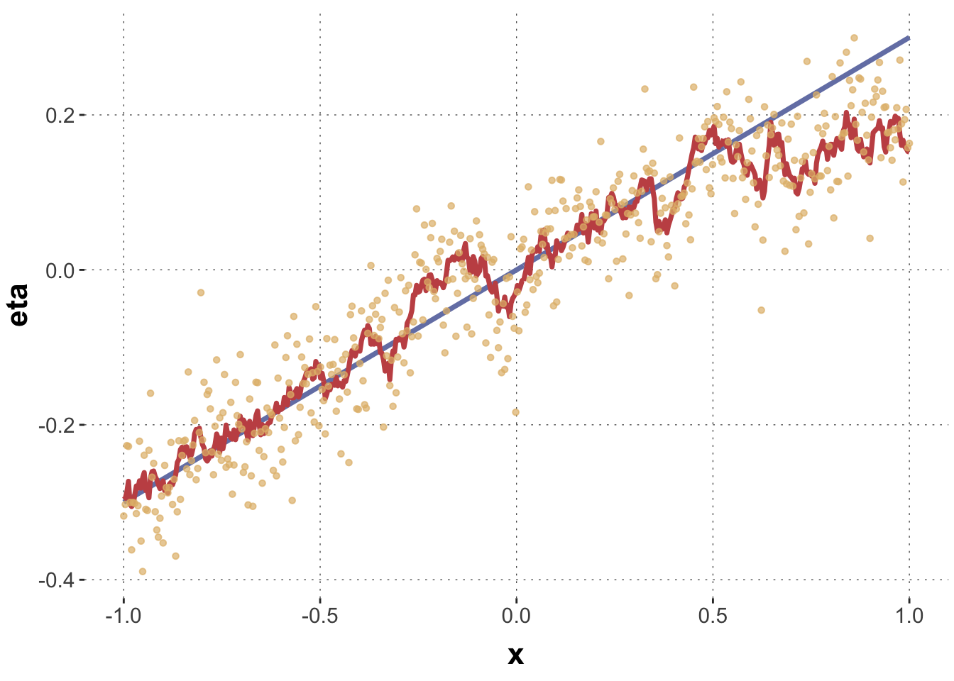
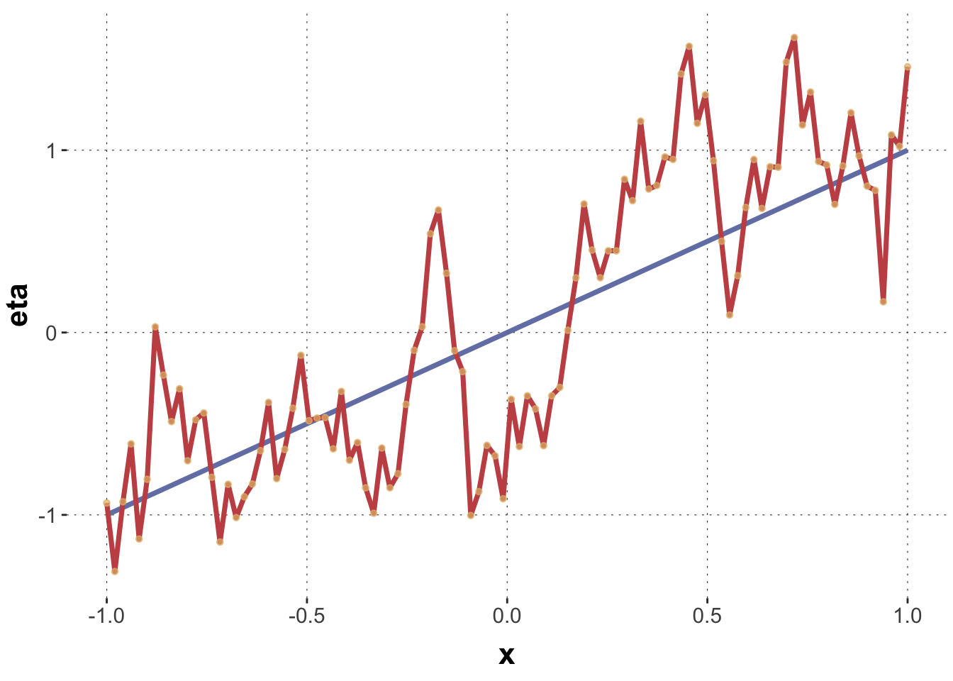
The blue line is a regular, simple linear regression line, the linear predictor part, if you will. The red line is the predictor of central tendency, obtained by overlaying the linear predictor with “wiggles” sampled from the Gaussian process. The yellow dots are actual samples (obtained from a normal distribution) around the central predictor line.

Exercise

Using these functions get intuitions for the kinds of curves you generate for different input vectors and parameter constellations.

Caveat. This generation script is a simplified procedural illustration of a Gaussian process regression (an intuition gym). The actual implementation of a Bayesian Gaussian process regression (e.g., in brms) is much more involved. Nevertheless, we can appreciate the most important idea: for a set of parameter values supplied to the function get_GP_simulation we get different wiggly regression lines. So, reverting this generative process (or one similar to it), we can ask: which parameter values are likely to have generated a set of \(x,y\) observations? And that is the simple and elegant idea behing Bayesian Gaussian process regression.

GP regression in `brms`

To implement GP regression in brms (using a radial basis function kernel; the only kernel currently implemented), just need to specify gp() for the predictor for which we want “GP wiggles”, so to speak.

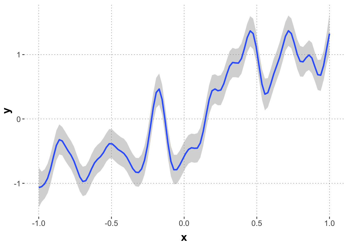
In practice, GPR can be slow and parameters hard to identify. Let’s therefore try a simple example of parameter recovery, keeping in mind that the underyling implementation in brms may be slightly different from the heuristic protocol used for intuition-building here. It will therefore be particularly interesting to see if we can recover the intercept and slope of the generating model, i.e., the “linear core” from which we are most likely to draw relevant conclusions eventually (e.g., is there a main (linear) effect of factor XYZ underneath the wiggliness).

Toggle code

GP_simulation <- get_GP_simulation(
  x = seq(-1,1, length.out = 100), 
  Intercept = 0, 
  slope = 1, 
  sigma_f = 0.5, 
  lambda  = 2, 
  sigma = 0.0001,
  seed = 1996)

plot_GP_simulation(GP_simulation)

Here is the GP-regression model in brms:

Toggle code

# results: hide
fit_GPR <- 
  brms::brm(
    formula = y ~ gp(x) + x,
    data    = GP_simulation,
    iter    = 4000
  )

It seems that we have recoverd the “linear core” parameters reasonably well, even if the estimates of the other parameter diverge from those we used to create the data (which is because the data-generating models are actually different).

Toggle code

summary(fit_GPR)

 Family: gaussian 
  Links: mu = identity; sigma = identity 
Formula: y ~ gp(x) + x 
   Data: GP_simulation (Number of observations: 100) 
  Draws: 4 chains, each with iter = 4000; warmup = 2000; thin = 1;
         total post-warmup draws = 8000

Gaussian Process Terms: 
            Estimate Est.Error l-95% CI u-95% CI Rhat Bulk_ESS Tail_ESS
sdgp(gpx)       0.44      0.08     0.32     0.61 1.00     1864     2144
lscale(gpx)     0.03      0.00     0.02     0.04 1.01      563      823

Population-Level Effects: 
          Estimate Est.Error l-95% CI u-95% CI Rhat Bulk_ESS Tail_ESS
Intercept     0.07      0.12    -0.16     0.30 1.00     3897     3082
x             1.16      0.19     0.80     1.55 1.00     4104     3568

Family Specific Parameters: 
      Estimate Est.Error l-95% CI u-95% CI Rhat Bulk_ESS Tail_ESS
sigma     0.21      0.02     0.17     0.25 1.00     2044     2958

Draws were sampled using sampling(NUTS). For each parameter, Bulk_ESS
and Tail_ESS are effective sample size measures, and Rhat is the potential
scale reduction factor on split chains (at convergence, Rhat = 1).

The fitted curve also looks very reasonable.

Toggle code

conditional_effects(fit_GPR)

Preamble

Gaussian processes

A compact prior over functions

GP regression in brms

GP regression in `brms`