MCMC diagnostics (demonstrations)

Bayesian regression: theory & practice

Author

Michael Franke

Preamble

Here is code to load (and if necessary, install) required packages, and to set some global options (for plotting and efficient fitting of Bayesian models).

Toggle code

# install packages from CRAN (unless installed)
pckgs_needed <- c(
  "tidyverse",
  "brms",
  "rstan",
  "rstanarm",
  "remotes",
  "tidybayes",
  "bridgesampling",
  "shinystan",
  "mgcv"
)
pckgs_installed <- installed.packages()[,"Package"]
pckgs_2_install <- pckgs_needed[!(pckgs_needed %in% pckgs_installed)]
if(length(pckgs_2_install)) {
  install.packages(pckgs_2_install)
} 

# install additional packages from GitHub (unless installed)
if (! "aida" %in% pckgs_installed) {
  remotes::install_github("michael-franke/aida-package")
}
if (! "faintr" %in% pckgs_installed) {
  remotes::install_github("michael-franke/faintr")
}
if (! "cspplot" %in% pckgs_installed) {
  remotes::install_github("CogSciPrag/cspplot")
}

# load the required packages
x <- lapply(pckgs_needed, library, character.only = TRUE)
library(aida)
library(faintr)
library(cspplot)

# these options help Stan run faster
options(mc.cores = parallel::detectCores())

# use the CSP-theme for plotting
theme_set(theme_csp())

# global color scheme from CSP
project_colors = cspplot::list_colors() |> pull(hex)
# names(project_colors) <- cspplot::list_colors() |> pull(name)

# setting theme colors globally
scale_colour_discrete <- function(...) {
  scale_colour_manual(..., values = project_colors)
}
scale_fill_discrete <- function(...) {
   scale_fill_manual(..., values = project_colors)
}

Toggle code

dolphin <- aida::data_MT
my_scale <- function(x) c(scale(x))

This tutorial provides demonstrations of how to check the quality of MCMC samples obtained from brms model fits.

A good model

To have something to go on, here are two model fits, one of this is good, the other is … total crap. The first model fits a smooth line to the average world temperature. (We need to set the seed here to have reproducible results.)

Toggle code

fit_good <- brm(
  formula = avg_temp ~ s(year), 
  data = aida::data_WorldTemp,
  seed = 1969
)

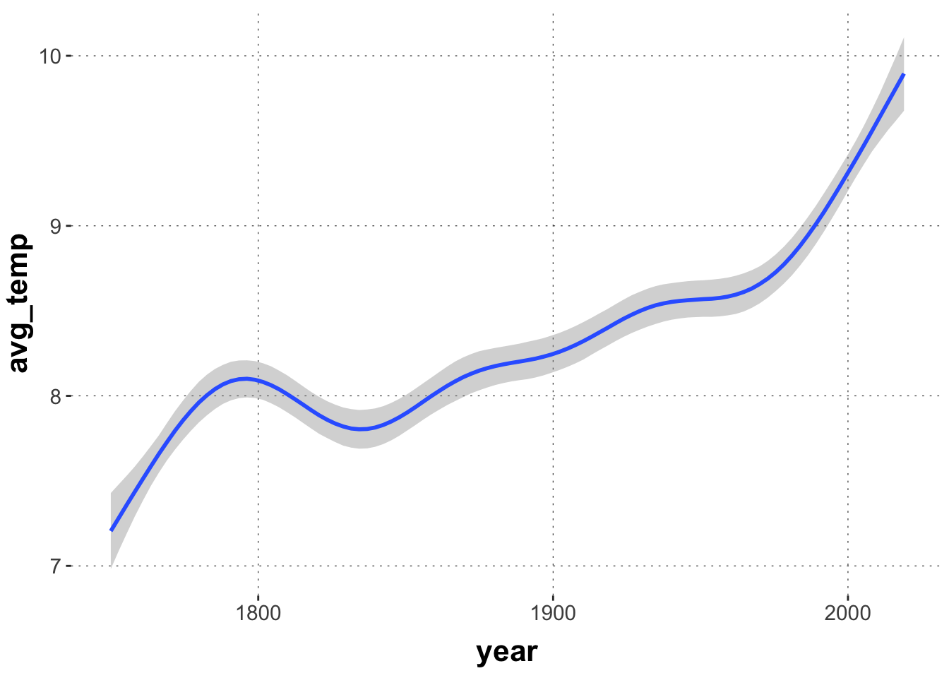
Here is a quick visualization of the model’s posterior prediction:

Toggle code

conditional_effects(fit_good)

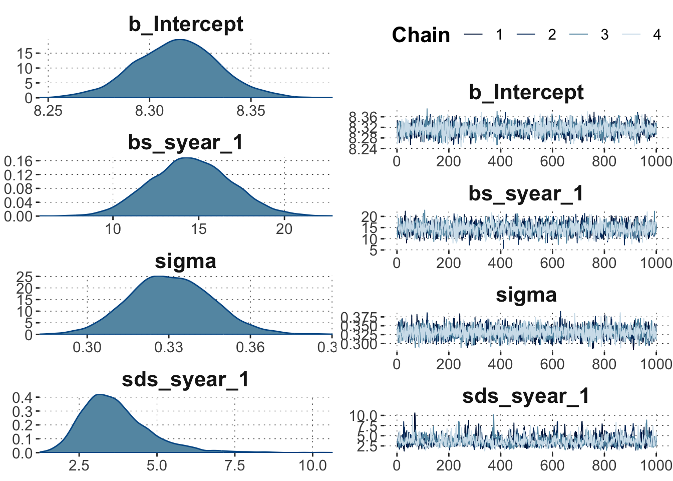
The good model is rather well behaved. Here is a generic plot of its posterior fits and traceplots:

Toggle code

plot(fit_good)

Traceplots look like hairy caterpillar madly-in-love with each other. The world is good.

We can check \(\hat{R}\) and effective sample sizes also in the summary of the model:

Toggle code

summary(fit_good)

 Family: gaussian 
  Links: mu = identity; sigma = identity 
Formula: avg_temp ~ s(year) 
   Data: aida::data_WorldTemp (Number of observations: 269) 
  Draws: 4 chains, each with iter = 2000; warmup = 1000; thin = 1;
         total post-warmup draws = 4000

Smooth Terms: 
             Estimate Est.Error l-95% CI u-95% CI Rhat Bulk_ESS Tail_ESS
sds(syear_1)     3.68      1.12     2.01     6.31 1.00     1070     1610

Population-Level Effects: 
          Estimate Est.Error l-95% CI u-95% CI Rhat Bulk_ESS Tail_ESS
Intercept     8.31      0.02     8.27     8.35 1.00     3759     2821
syear_1      14.56      2.34    10.14    19.13 1.00     2005     2552

Family Specific Parameters: 
      Estimate Est.Error l-95% CI u-95% CI Rhat Bulk_ESS Tail_ESS
sigma     0.33      0.02     0.30     0.36 1.00     2944     2567

Draws were sampled using sampling(NUTS). For each parameter, Bulk_ESS
and Tail_ESS are effective sample size measures, and Rhat is the potential
scale reduction factor on split chains (at convergence, Rhat = 1).

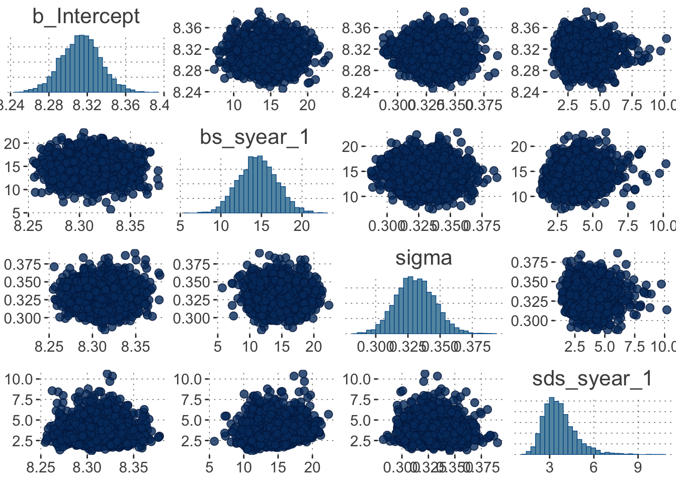
Importantly, the summary of the model contains a warning message about one divergent transition. We are recommended to check the pairs() plot, so here goes:

Toggle code

pairs(fit_good)

This is actually not too bad. (Wait until you see a terrible case below!)

We can try to fix this problem with a single divergent transition by doing as recommended by the warning message, namely increasing the adapt_delta parameter in the control structure:

Toggle code

fit_good_adapt <- brm(
  formula = avg_temp ~ s(year), 
  data = aida::data_WorldTemp,
  seed = 1969,
  control = list(adapt_delta=0.9),
) 

summary(fit_good_adapt)

 Family: gaussian 
  Links: mu = identity; sigma = identity 
Formula: avg_temp ~ s(year) 
   Data: aida::data_WorldTemp (Number of observations: 269) 
  Draws: 4 chains, each with iter = 2000; warmup = 1000; thin = 1;
         total post-warmup draws = 4000

Smooth Terms: 
             Estimate Est.Error l-95% CI u-95% CI Rhat Bulk_ESS Tail_ESS
sds(syear_1)     3.67      1.15     2.04     6.49 1.00      886     1311

Population-Level Effects: 
          Estimate Est.Error l-95% CI u-95% CI Rhat Bulk_ESS Tail_ESS
Intercept     8.31      0.02     8.27     8.35 1.00     3524     2788
syear_1      14.57      2.30    10.23    19.18 1.00     2137     2321

Family Specific Parameters: 
      Estimate Est.Error l-95% CI u-95% CI Rhat Bulk_ESS Tail_ESS
sigma     0.33      0.02     0.30     0.36 1.00     2703     2301

Draws were sampled using sampling(NUTS). For each parameter, Bulk_ESS
and Tail_ESS are effective sample size measures, and Rhat is the potential
scale reduction factor on split chains (at convergence, Rhat = 1).

That looks better, but what did we just do? — When the sampler “warms up”, it tries to find good parameter values for the case at hand. The adapt_delta parameter is the minimum amount of accepted proposals (where to jump next) before “warm up” counts as done and successfull. So with a small problem like this, just making the adaptation more ambitious may have have solved the problem. It has also, however, made the sampling slower, less efficient.

A powerful interactive tool for exploring a fitted model (diagnostics and more) is shinystan:

Toggle code

shinystan::launch_shinystan(fit_good_adapt)

A terrible model

The main (maybe only) reason for serious problems with the NUTS sampling is this: sampling issues arise for bad models. So, let’s come up with a really stupid model.

Here’s a model that is like the previous but adds a second predictor., This second predictor is intended to be a normal (non-smoothed) regression coefficient that is almost identical to the original year information. You may already intuit that this cannot possibly be a good idea; the model is notionally deficient. So, we expect nightmares during sampling:

Toggle code

fit_bad <-
  brms::brm(
  formula = avg_temp ~ s(year) + year_perturbed, 
  data = aida::data_WorldTemp |> mutate(year_perturbed = rnorm(1,year,0.001)),
  seed = 1969
)

Exercise 2

This model is deliberately set up to be stupid (and to mislead you). If you don’t like being held in the dark, try to find the mistake already.

Solution

See below.

Toggle code

summary(fit_bad)

 Family: gaussian 
  Links: mu = identity; sigma = identity 
Formula: avg_temp ~ s(year) + year_perturbed 
   Data: mutate(aida::data_WorldTemp, year_perturbed = rnor (Number of observations: 269) 
  Draws: 4 chains, each with iter = 2000; warmup = 1000; thin = 1;
         total post-warmup draws = 4000

Smooth Terms: 
             Estimate Est.Error l-95% CI u-95% CI Rhat Bulk_ESS Tail_ESS
sds(syear_1)     3.62      1.08     2.03     6.18 1.00     1171     1682

Population-Level Effects: 
                        Estimate         Est.Error           l-95% CI
Intercept      -2693691333829.80 12145265317737.51 -37056374746302.24
year_perturbed     1539251474.03     6940148378.55     -7252904977.78
syear_1                    14.61              2.34              10.19
                        u-95% CI Rhat Bulk_ESS Tail_ESS
Intercept      12692589621258.01 2.94        5       12
year_perturbed    21175061423.71 2.94        5       12
syear_1                    19.36 1.00     2769     2729

Family Specific Parameters: 
      Estimate Est.Error l-95% CI u-95% CI Rhat Bulk_ESS Tail_ESS
sigma     0.33      0.01     0.30     0.36 1.00     3642     2568

Draws were sampled using sampling(NUTS). For each parameter, Bulk_ESS
and Tail_ESS are effective sample size measures, and Rhat is the potential
scale reduction factor on split chains (at convergence, Rhat = 1).

Indeed, that looks pretty bad. We managed to score badly on all major accounts:

large \(\hat{R}\)
extremely poor efficient sample size
ridiculously far ranging posterior estimates for the main model components
tons of divergent transitions
maximum treedepth reached more often than hipster touches their phone in a week

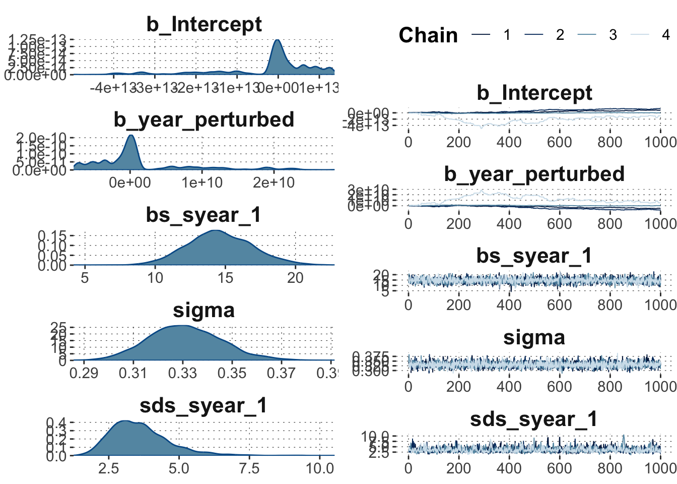
Some of these caterpillars look like they are in a vicious rose war:

Toggle code

plot(fit_bad)

We also see that that the intercept of and the slope for year_perturbed are the main troublemakers (in terms of traceplots).

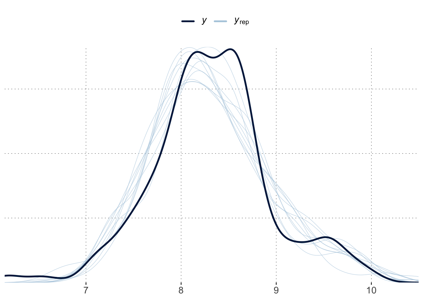
Interestingly, a simple posterior check doesn’t look too bad:

Toggle code

pp_check(fit_bad)

This shows that the warning messages (from Stan) shoult be taken seriously. The samples cannot be trusted, even if a posterior predictive check looks agreeable.

Exercise 1

Extract information about \(\hat{R}\) and the ratio of efficient samples with functions brms::rhat and brms::neff_ratio.

Interpret what you see: why are these numbers not good.

Solution

For R-hat, we do:

Toggle code

brms::rhat(fit_bad)

     b_Intercept b_year_perturbed       bs_syear_1      sds_syear_1 
       2.9426863        2.9426863        1.0025218        1.0037162 
           sigma     s_syear_1[1]     s_syear_1[2]     s_syear_1[3] 
       1.0007585        1.0018977        1.0006639        1.0020012 
    s_syear_1[4]     s_syear_1[5]     s_syear_1[6]     s_syear_1[7] 
       1.0005904        1.0012444        1.0005373        1.0005873 
    s_syear_1[8]           lprior             lp__ 
       0.9999082        1.0037192        1.0047583

These numbers are bad, since they ought to be close to 1, which is the ideal case when chains are indistinguishable (roughly put).

For the efficient-sample ratio:

Toggle code

brms::neff_ratio(fit_bad)

     b_Intercept b_year_perturbed       bs_syear_1      sds_syear_1 
     0.001153224      0.001153224      0.682138561      0.292844859 
           sigma     s_syear_1[1]     s_syear_1[2]     s_syear_1[3] 
     0.641937607      0.645693901      0.521896532      0.756250723 
    s_syear_1[4]     s_syear_1[5]     s_syear_1[6]     s_syear_1[7] 
     0.585514962      0.790196797      0.832935697      0.678273027 
    s_syear_1[8]           lprior             lp__ 
     0.790823858      0.293125594      0.242826922

These numbers are also poor, because we would like them, ideally, to be 1. However, low efficiency of samples is not necessary a sign that the fit cannot be trusted, just that the sampler has a hard time beating autocorrelation.

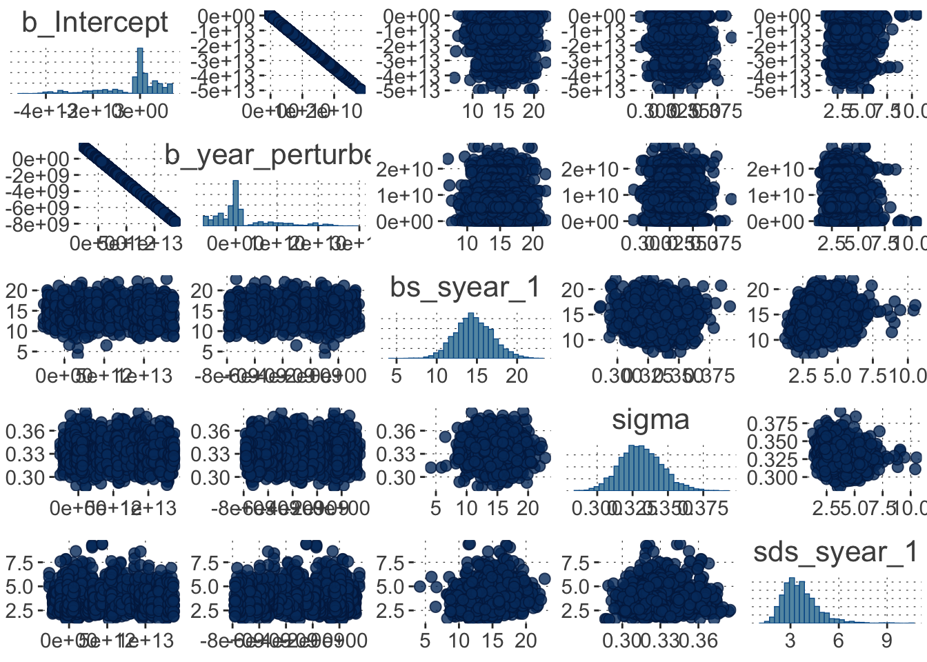
Have a look at the pairs() plot:

Toggle code

pairs(fit_bad)

Aha, there we see a clear problem! The joint posterior for the intercept and the slope for year_perturbed looks like a line. This means that these parameters could in principle do the same “job”.

This suggests a possible solution strategy. The model is too unconstrained. It can allow these two parameters meander to wherever they want (or so it seems). We could therefore try honing them in by specifying priors, like so:

Toggle code

fit_bad_wPrior <- brm(
  formula = avg_temp ~ s(year) + year_perturbed, 
  data = aida::data_WorldTemp |> mutate(year_perturbed = rnorm(1,year,0.001)),
  seed = 1969,
  prior = prior("student_t(1,0,5)", coef = "year_perturbed")
) 

summary(fit_bad_wPrior)

 Family: gaussian 
  Links: mu = identity; sigma = identity 
Formula: avg_temp ~ s(year) + year_perturbed 
   Data: mutate(aida::data_WorldTemp, year_perturbed = rnor (Number of observations: 269) 
  Draws: 4 chains, each with iter = 2000; warmup = 1000; thin = 1;
         total post-warmup draws = 4000

Smooth Terms: 
             Estimate Est.Error l-95% CI u-95% CI Rhat Bulk_ESS Tail_ESS
sds(syear_1)     3.61      1.09     1.93     6.17 1.01      774     1324

Population-Level Effects: 
               Estimate Est.Error  l-95% CI u-95% CI Rhat Bulk_ESS Tail_ESS
Intercept       1710.68  56636.65 -67751.31 74280.43 1.01     3201      846
year_perturbed    -0.97     32.36    -42.44    38.72 1.01     3201      846
syear_1           14.39      2.32      9.84    18.86 1.00     2122     1889

Family Specific Parameters: 
      Estimate Est.Error l-95% CI u-95% CI Rhat Bulk_ESS Tail_ESS
sigma     0.33      0.01     0.30     0.36 1.00     3433     2978

Draws were sampled using sampling(NUTS). For each parameter, Bulk_ESS
and Tail_ESS are effective sample size measures, and Rhat is the potential
scale reduction factor on split chains (at convergence, Rhat = 1).

Well, alright! That isn’t too bad anymore. But it is still clear from the posterior pairs plot that this model has two parameters that steal each other’s show. The model remains a bad model … for our data.

Toggle code

pairs(fit_bad)

Here’s what’s wrong: year_perturbed is a constant! The model is a crappy model of the data, because the data is not what we thought it would be. Check it out:

Toggle code

aida::data_WorldTemp |> mutate(year_perturbed = rnorm(1,year,0.001))

# A tibble: 269 × 5
    year anomaly uncertainty avg_temp year_perturbed
   <dbl>   <dbl>       <dbl>    <dbl>          <dbl>
 1  1750  -1.41        NA        7.20          1750.
 2  1751  -1.52        NA        7.09          1750.
 3  1753  -1.07         1.3      7.54          1750.
 4  1754  -0.614        1.09     8.00          1750.
 5  1755  -0.823        1.24     7.79          1750.
 6  1756  -0.547        1.28     8.06          1750.
 7  1757  -0.438        1.31     8.17          1750.
 8  1758  -2.42         1.76     6.19          1750.
 9  1759  -1.53         2.25     7.08          1750.
10  1760  -2.46         2.75     6.14          1750.
# ℹ 259 more rows

So, we basically ran a model with two intercepts!?! 😳

Let’s try again:

Toggle code

data_WorldTemp_perturbed <- aida::data_WorldTemp |> 
    mutate(year_perturbed = rnorm(nrow(aida::data_WorldTemp),year, 50))
data_WorldTemp_perturbed

# A tibble: 269 × 5
    year anomaly uncertainty avg_temp year_perturbed
   <dbl>   <dbl>       <dbl>    <dbl>          <dbl>
 1  1750  -1.41        NA        7.20          1705.
 2  1751  -1.52        NA        7.09          1753.
 3  1753  -1.07         1.3      7.54          1761.
 4  1754  -0.614        1.09     8.00          1769.
 5  1755  -0.823        1.24     7.79          1769.
 6  1756  -0.547        1.28     8.06          1758.
 7  1757  -0.438        1.31     8.17          1805.
 8  1758  -2.42         1.76     6.19          1752.
 9  1759  -1.53         2.25     7.08          1777.
10  1760  -2.46         2.75     6.14          1759.
# ℹ 259 more rows

That’s more like what we thought it was: year_perturbed is supposed to be noisy version of the actual year. So, let’s try again, leaving out the smoothing, just for some more chaos-loving fun:

Toggle code

fit_bad_2 <- brm(
  formula = avg_temp ~ year + year_perturbed, 
  data = data_WorldTemp_perturbed,
  seed = 1969,
  prior = prior("student_t(1,0,5)", coef = "year_perturbed")
) 

summary(fit_bad_2)

 Family: gaussian 
  Links: mu = identity; sigma = identity 
Formula: avg_temp ~ year + year_perturbed 
   Data: data_WorldTemp_perturbed (Number of observations: 269) 
  Draws: 4 chains, each with iter = 2000; warmup = 1000; thin = 1;
         total post-warmup draws = 4000

Population-Level Effects: 
               Estimate Est.Error l-95% CI u-95% CI Rhat Bulk_ESS Tail_ESS
Intercept         -3.50      0.58    -4.65    -2.37 1.00     3989     3346
year               0.01      0.00     0.01     0.01 1.00     3864     2228
year_perturbed     0.00      0.00    -0.00     0.00 1.00     3660     2684

Family Specific Parameters: 
      Estimate Est.Error l-95% CI u-95% CI Rhat Bulk_ESS Tail_ESS
sigma     0.41      0.02     0.37     0.44 1.00     1267     1130

Draws were sampled using sampling(NUTS). For each parameter, Bulk_ESS
and Tail_ESS are effective sample size measures, and Rhat is the potential
scale reduction factor on split chains (at convergence, Rhat = 1).

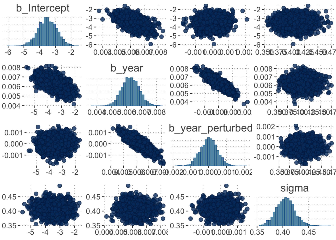
There are no warnings, so this model must be good, right? – No!

If we check the pairs plot, we see that we now have introduced a fair correlation between the two predictor variables.

Toggle code

pairs(fit_bad_2)

We should just not have year_perturbed; it’s nonsense, and it shows in the diagnostics.

You can diagnose more using shinystan:

Toggle code

shinystan::launch_shinystan(fit_bad)