Here is code to load (and if necessary, install) required packages, and to set some global options (for plotting and efficient fitting of Bayesian models).
Toggle code
# install packages from CRAN (unless installed)pckgs_needed <-c("tidyverse","brms","rstan","rstanarm","remotes","tidybayes","bridgesampling","shinystan","mgcv")pckgs_installed <-installed.packages()[,"Package"]pckgs_2_install <- pckgs_needed[!(pckgs_needed %in% pckgs_installed)]if(length(pckgs_2_install)) {install.packages(pckgs_2_install)} # install additional packages from GitHub (unless installed)if (!"aida"%in% pckgs_installed) { remotes::install_github("michael-franke/aida-package")}if (!"faintr"%in% pckgs_installed) { remotes::install_github("michael-franke/faintr")}if (!"cspplot"%in% pckgs_installed) { remotes::install_github("CogSciPrag/cspplot")}# load the required packagesx <-lapply(pckgs_needed, library, character.only =TRUE)library(aida)library(faintr)library(cspplot)# these options help Stan run fasteroptions(mc.cores = parallel::detectCores())# use the CSP-theme for plottingtheme_set(theme_csp())# global color scheme from CSPproject_colors = cspplot::list_colors() |>pull(hex)# names(project_colors) <- cspplot::list_colors() |> pull(name)# setting theme colors globallyscale_colour_discrete <-function(...) {scale_colour_manual(..., values = project_colors)}scale_fill_discrete <-function(...) {scale_fill_manual(..., values = project_colors)}
The “eight schools” example
The “eight schools” example (going back to Rubin (1981) is an often used simple illustration of a hierarchical model. There are \(N =8\) pairs of observations, each pair from a different school. For each school \(i\), we have an estimated effect size \(y_i\) and an estimated standard error \(\sigma_i\) for the reported effect size. (The experiments conducted at each school which gave us these pairs investigated whether short-term coaching has a effect on SAT-V scores, but this is not important for our purposes here.)
We are interested in inferring the latent true effect size \(\theta_i\) for each school \(i\) that could have generated the observed effect size \(y_i\) given spread \(\sigma_i\).
We could assume that each school’s true effect size \(\theta_i\) is entirely independent of any other. In contrast, we could assume that there is a single true effect size for all schools \(\theta_i = \theta_j\) for all \(i\) and \(j\). Or, more reasonably, we let the data decide and consider a model that tries to estimate how likely it is that \(\theta_i\) and \(\theta_j\) for different schools \(i\) and \(j\) are similar or not.
To do so, we assume a hierarchical model. The true effect sizes \(\theta_i\) and \(\theta_j\) of schools \(i\) and \(j\) are assumed:
to have played a role in (stochastically) generating the observed \(y_i\) and \(y_j\), and
to be themselves (stochastically) generated by (a hierarchical) process that generates (and thereby possibly assimilates) the values of \(\theta_i\) and \(\theta_j\).
Normally, there are a lot of divergent transitions when you run this code. This number can be retrieved (for stanfit objects, but not for brmsfit objects) with the function rstan::get_num_divergent():
Toggle code
rstan::get_num_divergent(stan_fit_8schoolsC)
[1] 48
Let’s go explore these divergent transitions using shinystan. Execute the command below, go to the tab “Explore” in the Shiny App, select “Bivariate” and explore plots of \(\sigma'\) against \(\theta_i\) for different \(i\). Points that experienced divergent transitions are shown in red.
Toggle code
shinystan::launch_shinystan(stan_fit_8schoolsC)
Divergent transition: where and why
The model has divergent transitions. But these are not random. They occur for specific samples. This gives us a clue as to why they arise.
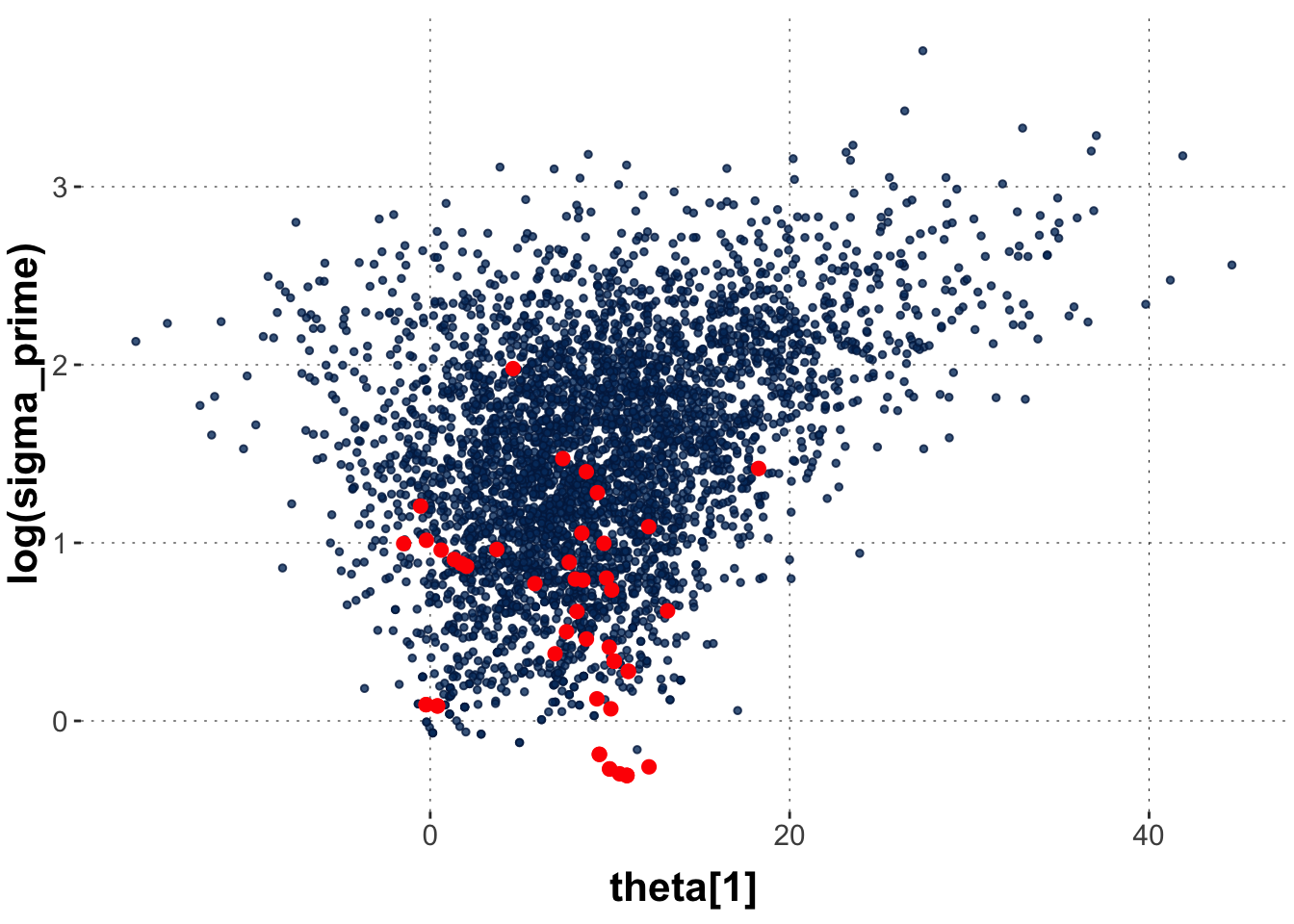
To see the regularity, here is a scatter plot of posterior samples from two parameters: \(\theta_1\) (arbitrary choice of index!) and \(\sigma'\). We use log-transforms of the latter for better visibility: Points with divergencies are shown in red.
This plot shape is also referred to as a “funnel” because it looks like, well, a funnel. We see now that the samples with divergencies actually happened mostly deep in the funnel. And that tells us something.
Since the step size parameter for approximating the Hamiltonian dynamics is set globally, we run into divergent transitions specifically for cases where \(\sigma'\) is very small (roughly \(<1\)), because for such smaller values of \(\sigma'\), the “reasonable” values for \(\theta_i\) are much more constrained / have lower variance than for higher values. That’s why the globally optimal step size leads to divergences inside the narrow part of the “funnel”.
A second model: non-centered parameterization
An alternative model, with so-called non-central parameterization does not have this problem with divergent transitions (or better: not that much of a problem; they can still occur occasionally even in this model).
To understand (intuitively) why is non-central paramterization more resilient against divergent, first recall the reason for the divergencies in the first model. Inside the funnel, so to speak, the variance of “good” \(\theta_i\) values were much smaller than outside of it. So, the sampler was not able to to flexibly accommodate differences in changes to \(\theta_i\) parameters as \(\sigma'\) changed. The non-central parameterization overcomes exactly this problem, because it decouples \(\sigma'\) and \(\theta_i\) via an additional parameter \(\eta_i\).
A heuristic way of seeing the crucial difference between models is that in the first (central parameterization) model, the distribution from which latent parameters are sampled depends itself on the value of sampled latent parameters, whereas in the second (non-central parameterization) model the distributions from which each latent parameter is sampled are fixed, i.e., independent from values of other parameters. Sampling from the latter is therefore easier to optimize.
Why care about divergent transitions?
We see why we should care about divergent transitions based on this simple example if we ask concretely:
What is the main striking difference (apart from the presence/absence of divergent transitions)?
How is this difference a reason for why divergent transitions can be problematic?
Is any estimated posterior mean for any parameter noticeably affected by this?
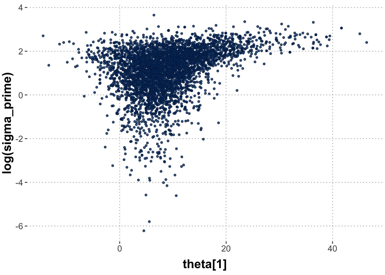
The “funnel” in the non-central model fit is much “deeper”. The samples for \(\log \sigma'\) stopped at around 1 for the first model with central-parameterization. But for the non-central one they go to values of -4. While this is in log-scale, it nevertheless shows how the divergencies can cause failure to explore a reasonable chunk of the posterior space. Expectations based on samples with such restrictions can consequently be biased. Indeed, the estimated mean for \(\sigma'\) is discernibly lower for the non-centralized parameterization.