Non-linear models in brms

Bayesian regression: theory & practice

It is possible to supply non-linear predictor terms in brms. These are of the form:

\[ \eta = X \beta + F(X', \theta_1, \dots, \theta_n) \]

where \(X'\) are the predictor terms feeding into non-linear function \(F\), with parameters \(\theta_1, \dots, \theta_n\). These parameters can themselves be predicted by linear terms, e.g., in the form:

\[ \theta_i = X'' \beta_{\theta_i} \]

Preamble

Here is code to load (and if necessary, install) required packages, and to set some global options (for plotting and efficient fitting of Bayesian models).

Toggle code

# install packages from CRAN (unless installed)
pckgs_needed <- c(
  "tidyverse",
  "brms",
  "rstan",
  "rstanarm",
  "remotes",
  "tidybayes",
  "bridgesampling",
  "shinystan",
  "mgcv"
)
pckgs_installed <- installed.packages()[,"Package"]
pckgs_2_install <- pckgs_needed[!(pckgs_needed %in% pckgs_installed)]
if(length(pckgs_2_install)) {
  install.packages(pckgs_2_install)
} 

# install additional packages from GitHub (unless installed)
if (! "aida" %in% pckgs_installed) {
  remotes::install_github("michael-franke/aida-package")
}
if (! "faintr" %in% pckgs_installed) {
  remotes::install_github("michael-franke/faintr")
}
if (! "cspplot" %in% pckgs_installed) {
  remotes::install_github("CogSciPrag/cspplot")
}

# load the required packages
x <- lapply(pckgs_needed, library, character.only = TRUE)
library(aida)
library(faintr)
library(cspplot)

# these options help Stan run faster
options(mc.cores = parallel::detectCores())

# use the CSP-theme for plotting
theme_set(theme_csp())

# global color scheme from CSP
project_colors = cspplot::list_colors() |> pull(hex)
# names(project_colors) <- cspplot::list_colors() |> pull(name)

# setting theme colors globally
scale_colour_discrete <- function(...) {
  scale_colour_manual(..., values = project_colors)
}
scale_fill_discrete <- function(...) {
   scale_fill_manual(..., values = project_colors)
}

Forgetting: power or exponential

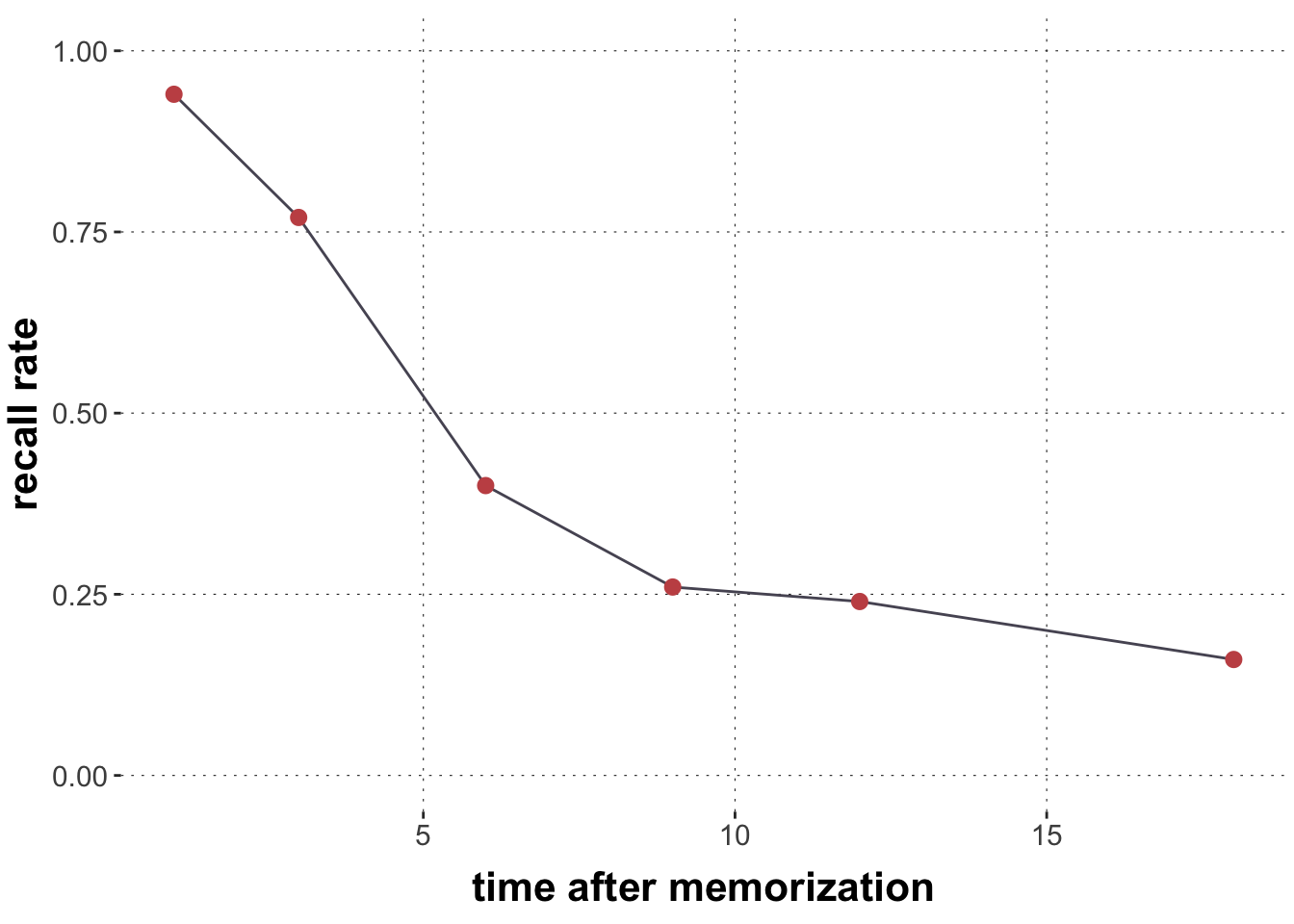
Here is a very small data set from (Murdoch 1961), as used in this tutorial paper on MLE. We have recall rates y for 100 subjects at six different time points t (in seconds) after after memorization:

Toggle code

data_forget <- tibble(
  y = c(.94, .77, .40, .26, .24, .16),
  t = c(  1,   3,   6,   9,  12,  18),
  N = 100,
  k = y * N
)

data_forget |>
  ggplot(aes(x = t, y = y)) +
  geom_line(color = project_colors[6]) +
  geom_point(color = project_colors[2], size = 2.5) +
  ylim(0,1) +
  xlab("time after memorization") +
  ylab("recall rate") 

There are two competing models on the table. The exponential model assumes that recall rates are predicted by exponential decay:

\[ \begin{align*} k & \sim \text{Binomial}( \theta, 100) \\ \theta &= a \exp (-bt) \\ a,b & \sim \text{log-Normal}(0, 0.5) \end{align*} \]

In contrast, the power model assumes that forgetting curves follow a power function:

\[ \begin{align*} k & \sim \text{Binomial}( \theta, 100) \\ \theta &= ct^{-d} \\ c,d &\sim \text{log-Normal}(0, 0.5) \end{align*} \]

We can think of these models as composed of a regular likelihood function (Binomial) with a non-linear predictor function \(F(x,y)\) (exponential or power), instead of the usual logistic-transformed linear predictor we know from logistic regression.

To define these non-linear models in brms, we use special syntax in the brmsformula. For the exponential model, for example, we use:

Toggle code

brms::bf(k | trials(N) ~ a * exp(-b * t), 
         a + b ~ 1, 
         nl=TRUE),

Noteworthy here is that we can define the regressor part as a Stan function, introducing hitherto unknown variables a and b, which we can then regress against liner predictor terms. Since in the currenct case, we only want to fit these two parameters, we write this like an intercept-only model. Importantly, we must declare the model explicitly as a non-linear model using the parameter nl=TRUE.

The full function call also specifies priors for the parameters a and b (notice the explicit setting of a lower bound at zero). We also must declare the likelihood function (Binomial) and the link function (here: identity, because the non-linear predictor is the expected value already; not need to transform it with another link function).

Toggle code

fit_exponential <- brms::brm(
    formula = brms::bf(k | trials(N) ~ a * exp(-b * t), 
                       a + b ~ 1, 
                       nl=TRUE),
    data    = data_forget,
    prior   = prior(lognormal(0,0.5), nlpar = "a", lb = 0) + 
              prior(lognormal(0,0.5), nlpar = "b", lb = 0),
    family  = binomial(link = "identity"),
    control = list(adapt_delta = 0.99)
  )

The power model is set-up in parallel.

Toggle code

fit_power <- brms::brm(
    formula = brms::bf(k | trials(N) ~ c * t^(-d), 
                       c + d ~ 1, 
                       nl=TRUE),
    data    = data_forget,
    prior   = prior(lognormal(0,0.5), nlpar = "c", lb = 0) + 
              prior(lognormal(0,0.5), nlpar = "d", lb = 0),
    family  = binomial(link = "identity"),
    control = list(adapt_delta = 0.99)
  )

Let’s try using leave-one-out cross-validation to address the question which model provides a fit to this data set.

Toggle code

loo_compare <- 
  loo_compare(
    loo(fit_exponential), 
    loo(fit_power))

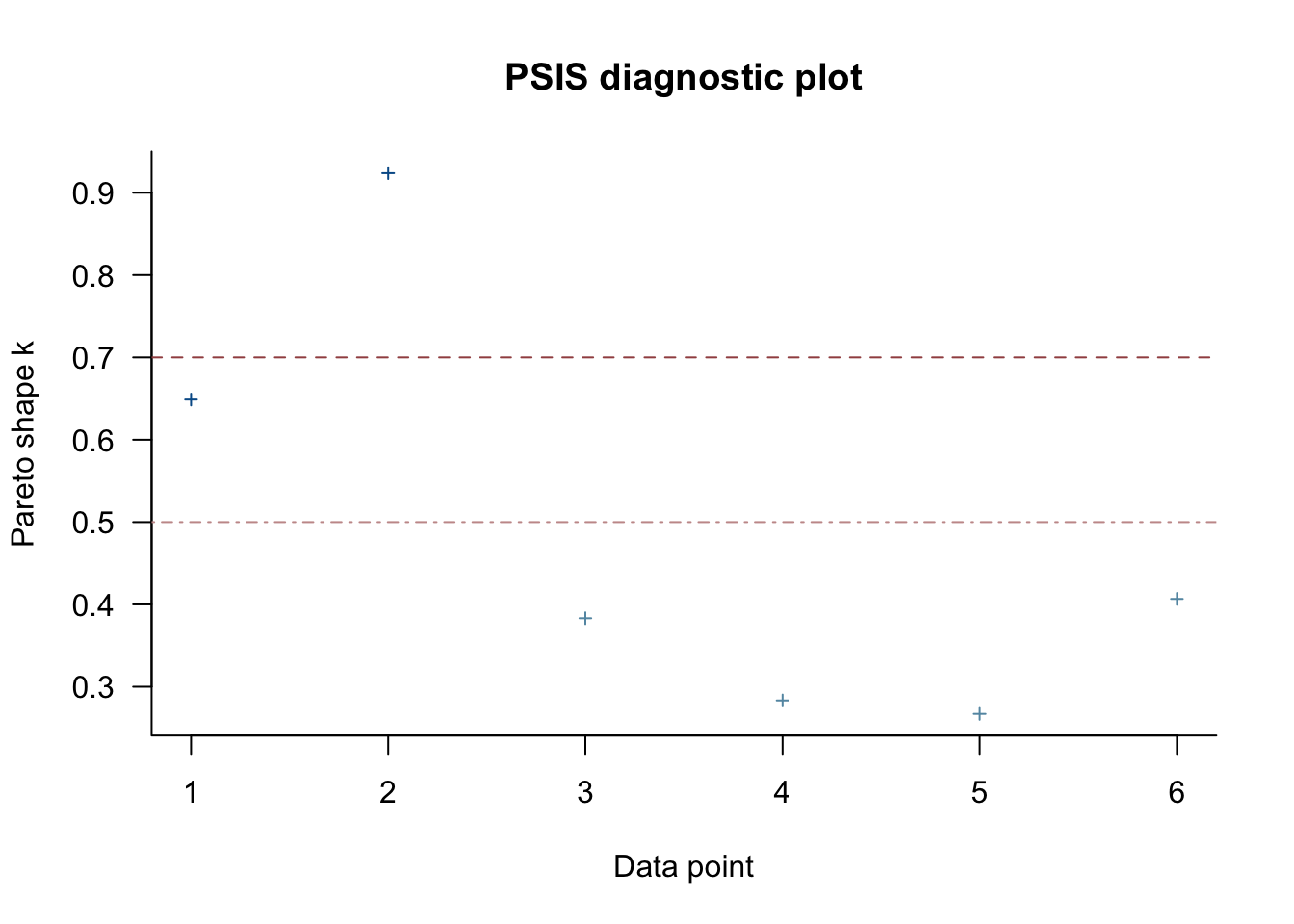
There is a problem. The loo function throws a warning that at least one observation is problematic under the Pareto-k diagnostic. We see that this is the first one:

Toggle code

plot(loo(fit_power))

But that plot also shows that we may have done something weird! We have treated as a single data point all 100 observations for each time step. No wonder that some of these observations heavily influence to total likelihood. These observations are huge chunks of atomic observations.

Let’s run these models again, but not as a Binomial model, but with a Bernoulli likelihood function, so that in LOO-based model comparison single observations are individual trials, not all trials from a given time point. Towards this end, we first unrol the data using uncount().

Toggle code

data_forget_long <- 
  data_forget |> 
  mutate(l = N-k) |> 
  dplyr::select(t,l,k) |> 
  pivot_longer(c(l,k), names_to = "y") |> 
  uncount(value) |> 
  mutate(y = ifelse(y == "k", TRUE, FALSE))

And then we fit the models again:

Toggle code

fit_exponential <- brms::brm(
    formula = brms::bf(y ~ a * exp(-b * t), 
                       a + b ~ 1, 
                       nl=TRUE),
    data    = data_forget_long,
    prior   = prior(lognormal(0,0.4), nlpar = "a", lb = 0) + 
              prior(lognormal(0,0.4), nlpar = "b", lb = 0),
    family  = bernoulli(link = "identity"),
    control = list(adapt_delta = 0.99)
  )

Toggle code

fit_power <- brms::brm(
    formula = brms::bf(y ~ c * t^(-d), 
                       c + d ~ 1, 
                       nl=TRUE),
    data    = data_forget_long,
    prior   = prior(lognormal(0,0.4), nlpar = "c", lb = 0) + 
              prior(lognormal(0,0.4), nlpar = "d", lb = 0),
    family  = bernoulli(link = "identity"),
    control = list(adapt_delta = 0.999)
  )

Now we can try the LOO-based model comparison again:

Toggle code

loo_comp <- 
  loo_compare(
    loo(fit_exponential), 
    loo(fit_power))
loo_comp

                elpd_diff se_diff
fit_exponential  0.0       0.0   
fit_power       -7.6       5.6   

That worked smoothly. The results show that the power model has a worse LOO-fit, and that the difference in expected log-probability density is substantial (a smaller standard error than the difference itself).

We may use Ben Lambert’s test for significance, just to out a number (a \(p\)-value) to it:

Toggle code

1- pnorm(-loo_compare[2,1], loo_comp[2,2])

[1] 0.0001370782

Exercise

Run a (linear) logistic regression model y ~ t and compare it to the two non-linear models with loo_compare. Interpret your results.

Solution

Toggle code

fit_logistic <- 
  brms::brm(
    formula = y ~ t,
    data    = data_forget_long,
    family  = bernoulli(link = "logit")
  )

Toggle code

loo_comp <- 
  loo_compare(
    list(
      loo(fit_logistic),
      loo(fit_exponential),
      loo(fit_power)
    ))
loo_comp

                elpd_diff se_diff
fit_exponential   0.0       0.0  
fit_power        -7.6       5.6  
fit_logistic    -16.2       4.3  

Models are ordered from better to worse. Differences are with respect to the best model (not the previous). We must therefore also compare the latter two directly:

Toggle code

loo_comp <- 
  loo_compare(
    list(
      loo(fit_logistic),
      loo(fit_power)
    ))
loo_comp

             elpd_diff se_diff
fit_power     0.0       0.0   
fit_logistic -8.6       8.3   

The non-linear power model and the linear logistic model seem to be on a par.

Toggle code

1- pnorm(-loo_compare[2,1], loo_comp[2,2])

[1] 0.1764362

The linear model seems slightly worse, but that difference may not be substantial.