Sheet 4.1: Non-linear regression (custom MLP)

Author: Michael Franke

In this tutorial, we will fit a non-linear regression, implemented as a multi-layer perceptron. First, we will implement it the hard way: coding the different layers in terms of explicitly spelled out matrix operations. In the next worksheet, we will see how the use of modules from PyTorch’ neural network package `torch.nn` helps us implement the model in a more efficient way. Going through the model entirely by hand, helps understand what is happening ’under the hood’ and also helps appreciating the high-level functionality provided by software like PyTorch.

Packages & global parameters

We will need to import the `torch` package for the main functionality. We specifically import the neural network functionalities from PyTorch as `nn`. We use this here only for the training loss function (MSE). In order to have a convenient handle, we load the `torch.nn.functional` package into variable `F`. We use this to pick up the activation function (ReLU) we will use for our neural network.

import torch
import torch.nn as nn
import torch.nn.functional as F
import numpy as np
import seaborn as sns
import pandas as pd
import matplotlib.pyplot as plt
# import sys
import warnings
warnings.filterwarnings('ignore')

We will also globally set the float precision to 64:

torch.set_default_dtype(torch.float64)

True model

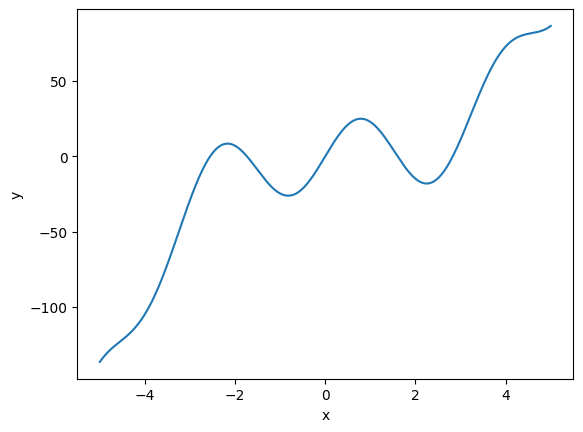
The “true model” is a constructed non-linear function \(y = f(x)\). Here is its definition and a plot to show what the “ground truth” looks like.

##################################################
## ground-truth model
##################################################

def goalFun(x):
    return(x**3 - x**2 + 25 * np.sin(2*x))

# create linear sequence (x) and apply goalFun (y)
x = np.linspace(start = -5, stop =5, num = 1000)
y = goalFun(x)

# plot the function
d = pd.DataFrame({'x' : x, 'y' : y})
sns.lineplot(data = d, x = 'x', y = 'y')
plt.show()

Training data

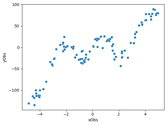
The training data consists of 100 pairs of \((x,y)\) values. Each pair is generated by first sampling an \(x\) value from a uniform distribution. For each sampled \(x\), we compute the value of the target function \(f(x)\) and add Gaussian noise to it.

##################################################
## generate training data (with noise)
##################################################

nObs = 100 # number of observations

# get noise around y observations
yNormal = torch.distributions.Normal(loc=0.0, scale=10)
yNoise  = yNormal.sample([nObs])

# get observations
xObs = 10*torch.rand([nObs])-5    # uniform from [-5,5]
yObs = xObs**3 - xObs**2 + 25 * torch.sin(2*xObs) + yNoise

# plot the data
d = pd.DataFrame({'xObs' : xObs, 'yObs' : yObs})
sns.scatterplot(data = d, x = 'xObs', y = 'yObs')
plt.show()

Exercise 4.1.1: Explore the training data

1. Remove the noise in the data by changing a single number (parameter value).

2. At what point is the noise in the data so large that there is nothing more to learn?

Hand-coding a multi-layer perceptron

Our model maps a single real number \(x\) onto another single real number \(y\). We therefore have a neural network whith input and output dimension set to 1. In between \(x\) and \(y\), we will use three hidden layers \(h_{1}, h_{2}, h_{3}\) each with dimension 10:

##################################################
## network dimension parameters
##################################################

nInput  = 1
nHidden = 10
nOutput = 1

The networks parameters are four matrices and four slopes. The first embedding is called \(U\), the following two hidden-to-hidden transformations are \(V_{1}\) and \(V_{2}\), the hidden-to-output mapping is given by matrix \(W\).

##################################################
## trainable (matrix & slope) parameters
##           --initializing weights --
##################################################

U  = torch.tensor(np.random.rand(nHidden,nInput)   * 2 - 1,
                  requires_grad=True)
V1 = torch.tensor(np.random.rand(nHidden, nHidden) * 2 - 1,
                  requires_grad=True)
V2 = torch.tensor(np.random.rand(nHidden, nHidden) * 2 - 1,
                  requires_grad=True)
W  = torch.tensor(np.random.rand(nOutput, nHidden) * 2 - 1,
                  requires_grad=True)
b1 = torch.zeros((nHidden,1), requires_grad=True)
b2 = torch.zeros((nHidden,1), requires_grad=True)
b3 = torch.zeros((nHidden,1), requires_grad=True)

Next, we will define the forward pass.

##################################################
## forward pass
##################################################

activationFun = F.relu # use ReLU fct from PyTorch

# this function takes a /single/ observation for x as input
#   and it outputs a /single/ observation for y
#   we will NOT use this one, but include for better understanding
def singleForwardPass(x):
    h1 = activationFun(U*x + b1)
    h2 = activationFun(torch.mm(V1,h1) + b2)
    h3 = activationFun(torch.mm(V2,h2) + b3)
    y  = torch.mm(W,h3)
    return(y[0,0])

# this function takes a /vector/ of observations for x as input
#   and it outputs a /vector/ of observations for y
#   we will use this function as it is massively more efficient in training
def singleForwardPassBatched(xObs):
    xObsBatched = xObs.reshape(100,1,1)       # 100 1x1 matrices
    h1 = activationFun(U @ xObsBatched + b1)  # 100 column vectors
    h2 = activationFun(V1 @ h1 + b2)
    h3 = activationFun(V2 @ h2 + b3)
    y  = W @ h3
    yReshaped = torch.reshape(y,(-1,))
    return(yReshaped)

Exercise 4.1.2: Digest the model, the parameters and their initialization

1. Verify that the functions ’singleForwardPass’ and ’singleForwardPassBatched’ do the same thing by comparing their predictions for the whole sequence of ’xObs’. I.e., simply call ’singleForwardPassBatched’ and compare the output to calls of ’singleForwardPass’. Ideally, produce outputs from ’singleForwardPass’ for all elements of ’xObs’ by list-comprehension.

2. Write down this model (forward pass) in mathematical notation. (The mathematical formulation of the model should follow the ’singleForwardPass’).

3. Describe the way parameters are initialized (above) in your own intuitive terms?

4. Why can we not just set all parameter values to 0 initially?

It remains to instantiate an optimizer and to run execute the training loop.

Next, we will define the ’forward pass’, i.e., a function that computes the predicted \(y\) for a given input \(x\) based on the current model parameters.

##################################################
## optimizer & training loop
##################################################

# initialize optimizer: Adam optimizer
loss_function = nn.MSELoss()
opt = torch.optim.Adam([U,V1,V2,W,b1,b2,b3], lr=1e-4)

epochs = 100000
for i in range(epochs+1):
    if (i == 0):
        print("\n")
    yPred = singleForwardPassBatched(xObs)
    loss  = loss_function(yPred, yObs)
    # loss  = torch.mean((yPred - yObs)**2)
    if (i == 0 or i % 5000 == 0):
        print('Iteration: {:5d} | Loss: {:12}'.format(i, loss.detach().numpy().round(0)))
        # print("Iteration: ", i, " Loss: ", loss.detach().numpy())
    loss.backward()
    opt.step()
    opt.zero_grad()

yPred = singleForwardPassBatched(xObs)

# plot the data
d = pd.DataFrame({'xObs' : xObs.detach().numpy(),
                  'yObs' : yObs.detach().numpy(),
                  'yPred': yPred.detach().numpy()})
dWide = pd.melt(d, id_vars = 'xObs', value_vars= ['yObs', 'yPred'])
sns.scatterplot(data = dWide, x = 'xObs', y = 'value', hue = 'variable', alpha = 0.7)
x = np.linspace(start = -5, stop =5, num = 1000)
y = goalFun(x)
plt.plot(x,y, color='g', alpha = 0.5)
plt.show()

#+begin_example


Iteration:     0 | Loss:       2730.0
Iteration:  5000 | Loss:        943.0
Iteration: 10000 | Loss:        630.0
Iteration: 15000 | Loss:        312.0
Iteration: 20000 | Loss:        168.0
Iteration: 25000 | Loss:        112.0
Iteration: 30000 | Loss:         79.0
Iteration: 35000 | Loss:         65.0
Iteration: 40000 | Loss:         61.0
Iteration: 45000 | Loss:         59.0
Iteration: 50000 | Loss:         59.0
Iteration: 55000 | Loss:         58.0
Iteration: 60000 | Loss:         58.0
Iteration: 65000 | Loss:         57.0
Iteration: 70000 | Loss:         57.0
Iteration: 75000 | Loss:         57.0
Iteration: 80000 | Loss:         57.0
Iteration: 85000 | Loss:         56.0
Iteration: 90000 | Loss:         56.0
Iteration: 95000 | Loss:         56.0
Iteration: 100000 | Loss:         55.0
#+end_example

Exercise 4.1.3: Inspecting and interpreting the model fit

0. [just for yourself] Make sure that you understand all ingredients and steps used here. Read up on the MSE loss function, for instance, or ask if you are unsure.

1. Inspect the print-outs from the training sequence. Does this output suggest that the training was successful or not?

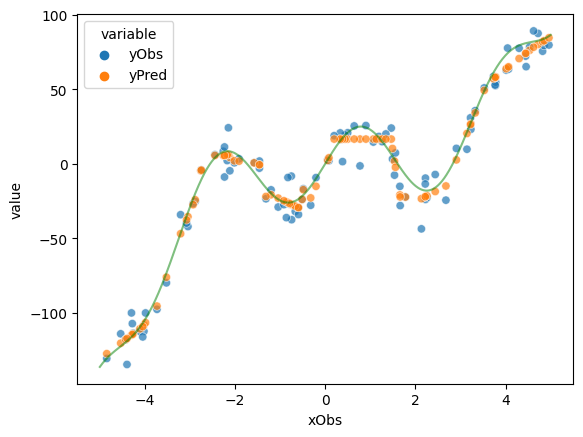
2. What does the plot produced here after training show exactly? Does that picture suggest that the model learned successfully? Do you think that there might even be a sense in which the model “overfitted” the data?

3. Change the optimizer to vanilla Gradient Descent (’SGD’), change the training rate to ’lr=1e-6’ and the number of training epochs to ’epochs = 50000’. Now, (first re-initialize all parameter values to start training anew) and repeatedly execute the last code cell (probably 4-6 times). Describe what you observe by answering the following questions: (i) is training with ’SGD’ more or less efficient than the initial set-up?; (ii) why is it more/less efficient? (iii) if we think of training the model as “curve fitting”, which parts of the curve are adapted first, which ones later? (iv) explain the difference you described in (iii).