Computing Bayes Factors
The goal of this post is to review a number of methods that approximate Bayes factors or marginalized likelihoods.
Model comparison by Bayes factors
A model , in the Bayesian sense, is a pair consisting of a conditional likelihood function for observable data together with a prior over parameter vector . Ideally, we might like to assess the absolute probability of model after seeing data . We can express this quantity using Bayes rule:
Quantifying over the whole class of possible models is dauntingly complex. This likely remains true even for a fixed data set and within a confined sub-genre of models (e.g., all regression models with combinations of a finite set of explanatory factors).
A good solution is to be more modest and to compare just two models to each other. The question to ask is then: How much does the observation of data impact our beliefs about the relative model probabilities? We can express this using Bayes rule as the ratio of our posterior beliefs about models, which eliminates the need to have the normalizing constant for the previous equation, like so:
The fraction on the left-hand side is the posterior odds ratio: our relative beliefs about models and after seeing data . On the right-hand side we have a product of two intuitively interpretable quantities. First, there is the prior odds: our relative beliefs about models and before seeing data . Second, there is the so-called Bayes factor. This way of introducing Bayes factors invites to think of them as the factor by which our prior odds change in the light of the data.
If the Bayes factor is close to 1, then data does little to change our relative beliefs. If the Bayes factor is large, say 100, then provides substantial evidence in favor of . Likewise, if it is small, say 0.01, then is relative evidence in favor of .
Marginal likelihoods
While Bayes factors are conceptually appealing, their computation can still be very complex. The quantity is often called the marginal likelihood. (It is also sometimes called the evidence but this usage of the term may be misleading because in natural language we usually refer to observational data as ‘evidence’; rather the Bayes factor is a plausible formalization of ‘evidence’ in favor of a model.) This term looks inoccuous but it is not. It can be a viciously complicated integral, because the likelihood of observation under the model must quantify over all possible parameters of that model, weighed as usual by their priors:
You may recognize in this integral the normalizing constant needed for parameter inference if we drop explicit reference to the specific model currently in focus:
Normally, we would like to avoid having to calculate the marginal likelihood, which is exactly why MCMC methods are so great: they approximate the posterior distribution over parameters without knowledge or computation of the marginal likelihood. This makes clear why computing Bayes factors, in general, can be quite difficult or a substantial computational burden.
Methods for Bayes factor computation
Two general approaches for computing or approximating Bayes factors can be distinguished. We can target the marginal likelihood of each model in separation. Or, we can target the Bayes factor directly. Both approaches have advantages and disadvantages, as we will see presently.
The following will spell out some methods for computing a Bayes factor. We apply these methods to the same models so that we can compare directly the results from each method and its results. The methods covered here are:
- Savage-Dickey density ratio (only applicable for nested models; see below)
- naive Monte Carlo sampling
- transdimensional MCMC
- supermodels
Data and full scripts (only the most important parts of which are shown here) are available for download.
The running-example model(s): Generalized Context Model
Chapter 17 of Lee & Wagenmakers’ (2014) textbook on Bayesian Cognitive Modeling features a concise implementation of the classic Generalized Context Model (GCM) of categorization. The model aims to predict the likelihood of correctly categorizing items after an initial learning period. Items differ along a number of numeric feature dimensions. (In the present case there will just be two categories and two feature dimensions.) The GCM revolves around three assumptions: (i) the probability of classifying item as belonging to category is derived from a measure of relative similarity of to all those items which were presented as belonging to category during training; (ii) similarity of any two items is a function of relative weighing of feature dimensions; (iii) there is room for general category preference (category is more likely to be chosen accross the board). (See chapter 17 of Lee & Wagenmakers and the papers cited therein for further details.)
In its simplest form, the model aims to predict the population-level category choices for nstim = 8 different stimuli. Category membership is stored in variable a = c(1,1,1,2,1,2,2,2), where an entry of 1 for the -th item means that it was presented as belonging to the first category during training. There are t = 320 trials in total (from different participants, but we do not distinguish these here.) The correct category choices (where correctness is determined by a) are stored in variable y = c(245, 218, 255, 126, 182, 71, 102, 65). Additionally, we supply two distance matrices d1 and d2 that give the distance between any two items along the two feature dimensions.
#################################################
## load & prepare data
#### data from Kruschke (1993)
#### taken from Lee & Wagenmakers (2014)
#################################################
load("KruschkeData.Rdata")
x <- y
y <- rowSums(x) # successful identifications per category
t <- n * nsubj  # number of trials
dataList <- list(y=y, nstim=nstim, t=t, a=a, d1=d1, d2=d2)
In the implementation of Lee & Wagenmakers, the GCM has three meaningful parameters, but we set the bias weight to b = 0.5:
- bias : overal bias in favor of one category over the other (there are only two categories in this case)
- attention weight : bias for weighing one feature dimension more strongly than the other (there are only two in this case)
- generalization strength : how much training items that are further away from the to-be-categorized item affect the current choice
A visualization of the model as a probabilistic dependency net is this (taken from Lee & Wagenmakers 2014, Chapter 17):
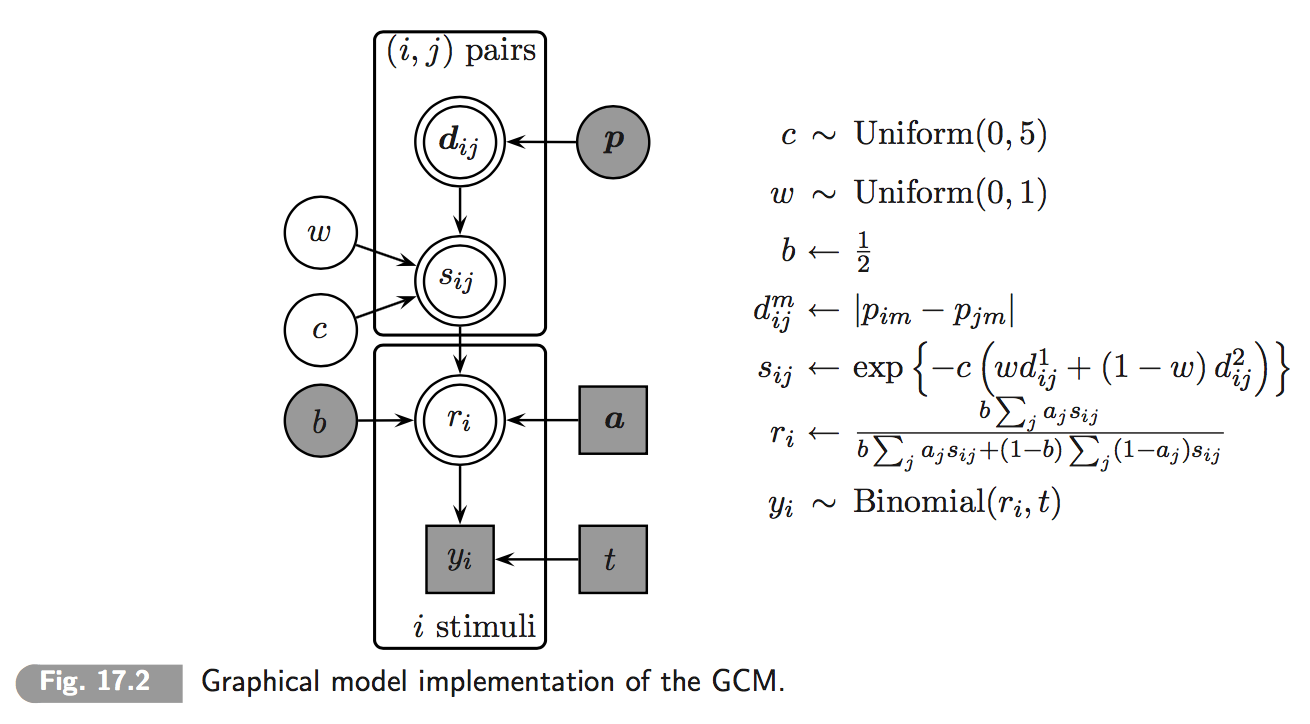
We are interested in comparing two models, both variants of the GCM. The first, more complex model is the one shown up here where weight has a flat prior over the unit interval w ~ dbeta(1,1). The second, simpler model is essentially the same but fixes the value of weight w = 0.5. This means that these models are so-called properly nested models and this, in turn, allows for computation of Bayes factors by the Savage-Dickey method.
Savage-Dickey density ratio
The Savage-Dickey density ratio method for calculating Bayes factors is particularly nice and elegant. An excellent tutorial on this method is [Wagenmakers et. al (2010)].
Unfortunately, the Savage-Dickey method only applies to properly nested models. Intuitively speaking, two models are nested if they are exactly alike but the parameter space of the nested model is a subset of the parameter space of the nesting model; they are properly nested if additional continuity assumptions of the prior over parameters hold. Concretely, model is properly nested under if:
- has parameters with vector free to vary;
- has parameters with set to fixed values;
- prior continuity: ;
- equal likelihood:
If models are properly nested we can compute the Bayes factor with the Savage-Dickey method as follows:
This seemingly magical result states that in order to compute the Bayes factor we only need to look at the ratio of the posterior of the parameters under the more complex model given data and the prior of under . To see that the above holds (the feeling of magic notwithstanding), here’s a proof sketch:
The above is a direct consequence of this last line.
Example: coin biases
Let’s illustrate the Savage-Dickey method with a simpler example for which we can also give an analytic solution for the Bayes factor. Suppose we observed k=7 successes in N=24 flips of a coin. The complex model has a likelihood function and a prior . The simpler (nested) model has the same likelihood function but fixes . We can then compute the Bayes factor in favor of the simpler as follows:
The Savage-Dickey method gives the same result:
This derivation uses the fact that the beta distribution is a conjugate prior for the binomial likelihood function, so that we can easily compute the posterior of after seeing for analytically, just using the beta distribution again. In general, starting with a prior the posterior over will be after seeing successes out of flips.
Savage-Dickey for the GCM example
Unlike for the previous simple coin-flip example, we do not know the precise mathematical form of the posterior over for the GCM. We can nonetheless use the Savage-Dickey method to approximate Bayes factors, by using an approximation of the posterior probability density for using samples from posterior distribution of . Posterior samples are here obtained using JAGS.
The JAGS code for the GCM looks like this (taken from Lee & Wagenmakers, 2014), and is stored in file GCM_1_posterior_inference.txt :
# JAGS code for the Generalized Context Model
model{
  # Decision Data
  for (i in 1:nstim){
    y[i] ~ dbin(r[i],t)
  }
  # Decision Probabilities
  for (i in 1:nstim){
    r[i] <- sum(numerator[i,])/sum(denominator[i,])
    for (j in 1:nstim){
      tmp1[i,j,1] <- b*s[i,j]
      tmp1[i,j,2] <- 0
      tmp2[i,j,1] <- 0
      tmp2[i,j,2] <- (1-b)*s[i,j]
      numerator[i,j] <- tmp1[i,j,a[j]]
      denominator[i,j] <- tmp1[i,j,a[j]] + tmp2[i,j,a[j]]
    }
  }
  # Similarities
  for (i in 1:nstim){
    for (j in 1:nstim){
      s[i,j] <- exp(-c*(w*d1[i,j]+(1-w)*d2[i,j]))
    }
  }
  # Priors
  c  ~ dunif(0,5)
  w  ~ dbeta(1,1)
  b <- 0.5
}
We will run the JAGS model through R. The code for doing so is contained in the file GCM_1_posterior_inference.R. First, we load some required packages:
library(tidyverse)
library(rjags)
library(ggmcmc)
library(polspline)
Then we run JAGS and retrieve 50000 samples of the posterior over after a burn-in of 15000, once for each of two chains.
modelFile = "GCM_1_posterior_inference.txt"jagsModel = jags.model(file = modelFile,
data = dataList, # dataList was defined above
n.chains = 2)
update(jagsModel, n.iter = 15000)
codaSamples = coda.samples(jagsModel,
variable.names = c("w"),
n.iter = 50000)
ms = ggs(codaSamples) # cast the data into tidy formatWe can then estimate the posterior density at , using the log-splines package:
post_samples = filter(ms, Parameter == "w")$value
fit.posterior <- logspline(post_samples, ubound=1, lbound=0)
posterior_w <- dlogspline(0.5, fit.posterior)
An approximation of the Bayes factor in favor of the complex model is then:
paste0("Approximate BF in favor of complex model (Savage-Dickey): ",
       round(1/posterior_w,3) )
## [1] "Approximate BF in favor of complex model (Savage-Dickey): 3.989"In sum, the Savage-Dickey method is an elegant and practical method for computing (or approximating, if based on sampling) Bayes factors for properly nested models. It is particularly useful when the nested model fixes just a small number of parameters that are free in the nesting model. The method needs to go through two bottlenecks that can introduce imprecision in an estimate: first, we may have to rely on posterior samples; second, we may have to rely an numerical approximation of a point-density from the samples.
Naive Monte Carlo simulation
While the Savage-Dickey method targets calculation of the Bayes factor directly, we can also target a single model’s marginal likelihood, as described above. Under certain circumstances (see end of this section for a critical assessment), even naive Monte Carlo simulation can work well and is very easy to implement when we already have a way of generating posterior samples, e.g., using an implementation in JAGS or similar software.
Naive Monte Carlo sampling approximates the marginal likelihood of model by sampling repeatedly parameter values from the prior and recording the likelihood of the data given the sampled parameter values. If we sample enough, the mean of the recorded likelihoods will approximate the true marginalized likelihood:
If we already have a JAGS implementation that produces samples from the posterior distribution, it only takes minor changes to obtain code that generates samples from the prior and returns the likelihood of the observed data. The following code, which is available in file GCM_2_BF_naiveMC.txt does exactly this. The crucial part is that we do not condition on the data; we take samples from the prior distribution. Instead we record (here: in variable lh) the log-likelihood of the observed data under each sample from the prior distribution.
# Generalized Context Model;
# version for naive MC sampling of marginal likelihood
model{
  # Decision Data
  for (i in 1:nstim){
    # y[i] ~ dbin(r[i],t) # commented out because we are
                          # NOT conditioning on data
    lhT[i] = dbin(y[i],r[i],t) # we track the likelihood of the data instead
  }
  lh = sum(log(lhT))
  # Decision Probabilities
  for (i in 1:nstim){
    r[i] <- sum(numerator[i,])/sum(denominator[i,])
    for (j in 1:nstim){
      tmp1[i,j,1] <- b*s[i,j]
      tmp1[i,j,2] <- 0
      tmp2[i,j,1] <- 0
      tmp2[i,j,2] <- (1-b)*s[i,j]
      numerator[i,j] <- tmp1[i,j,a[j]]
      denominator[i,j] <- tmp1[i,j,a[j]] + tmp2[i,j,a[j]]
    }
  }
  # Similarities
  for (i in 1:nstim){
    for (j in 1:nstim){
      s[i,j] <- exp(-c*(w*d1[i,j]+(1-w)*d2[i,j]))
    }
  }
  # Priors
  c  ~ dunif(0,5)
  w  ~ dbeta(betaParameter,betaParameter)
  b <- 0.5
}
Notice that the script also introduces a parameterization of the prior for w. This is handy because it allows us to use the same JAGS code for both models. (We need to compute the marginal likelihood for each model to obtain the Bayes factor estimate.)
The script in file GCM_2_BF_naiveMC.R approximate the marginal likelihood through naive Monte Carlo sampling. It’s major steps are reproduced here.
modelFile = "GCM_2_BF_naiveMC.txt"First, it defines a function that takes a betaParameter argument for the beta-prior over w to be fed to JAGS. The function returns 200,000 samples of the data’s likelihood under the prior.
nSamples = 200000
sample_likelihoods = function(betaParameter){
  # fix betaParameter for prior of w
  dataList$betaParameter = betaParameter
  # set up and run model
  jagsModel = jags.model(file = modelFile,
                         data = dataList,
                         n.chains = 2)
  update(jagsModel, n.iter = 15000)
  codaSamples = coda.samples(jagsModel,
                             variable.names = c("lh"),
                             n.iter = nSamples)
  # returns the sampled log likelihood values
  filter(ggs(codaSamples), Parameter == "lh")$value
}
To compute an approximate Bayes factor in this way, we call this function twice: once for the more complex, nesting model for which we set betaParameter = 1; and once for the simpler, nested model for which we approximate a fixed value of w = 0.5 simply by setting betaParameter = 50000. (This yields a very heavily peaked beta prior with mode at w=0.5 and should be good enough an approximation for our modest purposes.)
samples_complex = sample_likelihoods(betaParameter = 1)
samples_simple  = sample_likelihoods(betaParameter = 50000)
marg_lh_complex   = samples_complex %>% exp %>% mean
marg_lh_simple    = samples_simple  %>% exp %>% mean
The final result is reaonably close to the previous one from the Savage-Dickey method:
paste0("Approximate BF in favor of complex model (naive MC): ",
       round(marg_lh_complex/marg_lh_simple ,3))
## [1] "Approximate BF in favor of complex model (naive MC): 4.44"It is diagnostic to see the temporal development of the Bayes factor approximation as more and more samples are taken. This is plotted here, comparing it also to the result from the Savage-Dickey method (the red line).
BFVec = sapply(seq(10000,nSamples, by = 200),
               function(i) samples_complex[1:i] %>% exp %>% mean /
                           samples_simple[1:i]  %>% exp %>% mean)
ggplot(data.frame(i = seq(10000,nSamples, by = 200),
                  BF = BFVec),
       aes(x=i, y=BF)) +
  geom_line() +
  geom_hline(yintercept = 1/posterior_w,3, color = "firebrick") +
  xlab("number of samples") +
  ylab('approximate Bayes factor')
Transdimensional MCMC
A straightforward method for approximating posterior model odds is transdimensional MCMC. We consider the posterior over a binary model flag parameter which helps represent our prior and posterior beliefs about which of models and is true. We look at a single encompassing model that contains both models that are to be compared. The likelihood function of the encompassing model is switched between that of or depending on the current value of . A JAGS model that implements such an encompassing model is in the file GCM_3_BF_transdimensional.txt and reproduced here:
# Generalized Context Model
model{
  # Decision Data
  for (i in 1:nstim){
    y[i] ~ dbin(r[i],t)
    r[i] = ifelse(m == 0, r1[i], r2[i]) # which likelihood to
                                        # use depends on model flag
  }
  # Decision Probabilities
  for (i in 1:nstim){
    r1[i] <- sum(numerator1[i,])/sum(denominator1[i,])
    r2[i] <- sum(numerator2[i,])/sum(denominator2[i,])
    for (j in 1:nstim){
      tmp11[i,j,1] <- b1*s1[i,j]
      tmp12[i,j,1] <- b2*s2[i,j]
      tmp11[i,j,2] <- 0
      tmp12[i,j,2] <- 0
      tmp21[i,j,1] <- 0
      tmp22[i,j,1] <- 0
      tmp21[i,j,2] <- (1-b1)*s1[i,j]
      tmp22[i,j,2] <- (1-b2)*s2[i,j]
      numerator1[i,j] <- tmp11[i,j,a[j]]
      numerator2[i,j] <- tmp12[i,j,a[j]]
      denominator1[i,j] <- tmp11[i,j,a[j]] + tmp21[i,j,a[j]]
      denominator2[i,j] <- tmp12[i,j,a[j]] + tmp22[i,j,a[j]]
    }
  }
  # Similarities
  for (i in 1:nstim){
    for (j in 1:nstim){
      s1[i,j] <- exp(-c1*(w1*d1[i,j]+(1-w1)*d2[i,j]))
      s2[i,j] <- exp(-c2*(w2*d1[i,j]+(1-w2)*d2[i,j]))
    }
  }
  # Priors
  c1  ~ dunif(0,5)
  c2  ~ dunif(0,5)
  w1  ~ dbeta(1,1)
  w2  ~ dbeta(betaParameter,betaParameter)
  b1 <- 0.5
  b2 <- 0.5
  m ~ dbern(0.5) # model flag: prior odds are even
}
The script in file GCM_3_BF_transdimensional.R collects posterior samples from the model above.
modelFile = "GCM_3_BF_transdimensional.txt"All we really need to do is collect samples of the posterior over :
dataList$betaParameter = 50000
jagsModel = jags.model(file = modelFile,
                       data = dataList,
                       n.chains = 2)
update(jagsModel, n.iter = 75000)
codaSamples = coda.samples(jagsModel,
                           variable.names = c("m"),
                           n.iter = 250000)
Since we assumed that models are equally probable a priori (by taking ), the fraction of samples for which approximates the Bayes factor in favor of the complex model:
paste0("BF in favor of complex model (transcendental): ",
       round(1/mean(filter(ggs(codaSamples), Parameter == "m")$value) ,3))
## [1] "BF in favor of complex model (transcendental): 5.495"This method of estimation can be imprecise, especially when one model is much better than another. The intuitive reason is that whenever the MCMC chain sets , the parameters for model are free to meander wherever they like. This, in turn, makes it less likely that a proposal with is accepted. One possible solution to this is to use so-called pseudo-priors: set the priors for parameters of model to some function that resembles their posterior distribution when , but use the actual priors when .
Supermodels
A method similar to the previous promises to get around this problem, at least when the models’ marginal likelihoods are not too different. I will refer to this approach as ‘supermodels’ here, taking inspiration from this tutorial paper. Instead of a model flag, which determines which model’s likelihood function to use, we instead combine the model’s likelihoods in a linear way. Concretely, given parameter vectors and for models and respectively, we look at a model which contains both and and which has as the likelihood function of the data:
It is easy to show that for a flat prior , the posterior of is linear:
Since the posterior of is a distribution which satisfies , we get that . Since each model nested under the supermodel is a special case of either or we can use the Savage-Dickey method to express the posterior of as a function of only:
To obtain posterior samples from we use the JAGS code found in GCM_4_supermodels.txt.
modelFile = "GCM_4_supermodels.txt"The code is reproduced here:
# Generalized Context Model
data{
  one = 1
  zero = 0
  C = 1000000
}
model{
  # Decision Data
  for (i in 1:nstim){
    lh1[i] = dbin(y[i],r1[i],t)
    lh2[i] = dbin(y[i],r2[i],t)
  }
  # one ~ dbern(alpha * prod(lh1) + (1-alpha) * prod(lh2))
  zero ~ dpois(-log(alpha * prod(lh1) + (1-alpha) * prod(lh2)) + C)
  # Decision Probabilities
  for (i in 1:nstim){
    r1[i] <- sum(numerator1[i,])/sum(denominator1[i,])
    r2[i] <- sum(numerator2[i,])/sum(denominator2[i,])
    for (j in 1:nstim){
      tmp11[i,j,1] <- b1*s1[i,j]
      tmp12[i,j,1] <- b2*s2[i,j]
      tmp11[i,j,2] <- 0
      tmp12[i,j,2] <- 0
      tmp21[i,j,1] <- 0
      tmp22[i,j,1] <- 0
      tmp21[i,j,2] <- (1-b1)*s1[i,j]
      tmp22[i,j,2] <- (1-b2)*s2[i,j]
      numerator1[i,j] <- tmp11[i,j,a[j]]
      numerator2[i,j] <- tmp12[i,j,a[j]]
      denominator1[i,j] <- tmp11[i,j,a[j]] + tmp21[i,j,a[j]]
      denominator2[i,j] <- tmp12[i,j,a[j]] + tmp22[i,j,a[j]]
    }
  }
  # Similarities
  for (i in 1:nstim){
    for (j in 1:nstim){
      s1[i,j] <- exp(-c1*(w1*d1[i,j]+(1-w1)*d2[i,j]))
      s2[i,j] <- exp(-c2*(w2*d1[i,j]+(1-w2)*d2[i,j]))
    }
  }
  # Priors
  c1  ~ dunif(0,5)
  c2  ~ dunif(0,5)
  w1  ~ dbeta(1,1)
  w2  ~ dbeta(betaParameter,betaParameter)
  b1 <- 0.5
  b2 <- 0.5
  alpha ~ dbeta(1,1)
}
Since JAGS only allows sampling from or conditioning by distributions that it knows, we need to use the zero trick (alternatively: the one trick) to implement our custom linear-combination likelihood function.
We then collect samples from the posterior of :
jagsModel = jags.model(file = modelFile,
                       data = dataList,
                       n.chains = 2)
update(jagsModel, n.iter = 75000)
codaSamples = coda.samples(jagsModel,
                           variable.names = c("alpha"),
                           n.iter = 250000)
Subsequently, we obtain a point-estimate for the best-fitting that may have generated these posterior samples and compute the Bayes factor from it with the following function:
get_BF = function(alpha) {
  nll = Vectorize(function(c) {
    - sum(log(2*(1-c) * alpha + c))
  })
  c = optim(par = list(c = 0.1),
            fn = nll,
            lower = 0.000000001,
            method = "L-BFGS-B")$par
  (2-c)/c
}
This gives us another estimate of the Bayes factor:
paste0("BF in favor of complex model (supermodels): ",
       round(get_BF(filter(ggs(codaSamples), Parameter == "alpha")$value) ,3))
## [1] "BF in favor of complex model (supermodels): 4.443"Summary
The estimated Bayes factors all differed to a certain extent. The quality of the estimates could be enhanced by taking more samples in each case. Estimates that additionally depend on later approximate computations are generally less preferred. For example, we used logsplines to estimate the posterior density at a point based on MCMC samples for the Savage-Dickey method; we looked at the maximum likelihood estimate for intercept in the supermodels approach. My impression is that the most workable and scalable methods are those that approximate marginal likelihoods individually and do not require post-sampling approximations. Here, only naive MC sampling was covered. A great recent tutorial for more sophisticated methods can be found here. In sum, although I like the supermodels approach best (conceptual elegance!), currently my money is on bridge sampling whenever a model does not allow for a brute force method like grid approximation or naive MC sampling.