- basics
- joint distributions & marginalization
- conditional probability & Bayes rule
- 3 pillars of Bayesian data analysis:
- estimation
- comparison
- prediction
- parameter estimation for coin flips
- conjugate priors
- highest density interval
\[ \definecolor{firebrick}{RGB}{178,34,34} \newcommand{\red}[1]{{\color{firebrick}{#1}}} \] \[ \definecolor{mygray}{RGB}{178,34,34} \newcommand{\mygray}[1]{{\color{mygray}{#1}}} \] \[ \newcommand{\set}[1]{\{#1\}} \] \[ \newcommand{\tuple}[1]{\langle#1\rangle} \] \[\newcommand{\States}{{T}}\] \[\newcommand{\state}{{t}}\] \[\newcommand{\pow}[1]{{\mathcal{P}(#1)}}\]
key notions
recap
definition of conditional probability:
\[P(X \, | \, Y) = \frac{P(X \cap Y)}{P(Y)}\]
definition of Bayes rule:
\[P(X \, | \, Y) = \frac{P(Y \, | \, X) \ P(X)}{P(Y)}\]
version for data analysis:
\[\underbrace{P(\theta \, | \, D)}_{posterior} \propto \underbrace{P(\theta)}_{prior} \ \underbrace{P(D \, | \, \theta)}_{likelihood}\]
Bayes rule in multi-D
proportions of eye & hair color
joint probability distribution as a two-dimensional matrix:
knitr::kable(prob2ds)
| blond | brown | red | black | |
|---|---|---|---|---|
| blue | 0.03 | 0.04 | 0.00 | 0.41 |
| green | 0.09 | 0.09 | 0.05 | 0.01 |
| brown | 0.04 | 0.02 | 0.09 | 0.13 |
marginal distribution over eye color:
rowSums(prob2ds)
##  blue green brown
##  0.48  0.24  0.28
proportions of eye & hair color
joint probability distribution as a two-dimensional matrix:
prob2ds
##       blond brown  red black
## blue   0.03  0.04 0.00  0.41
## green  0.09  0.09 0.05  0.01
## brown  0.04  0.02 0.09  0.13
conditional probability given blue eyes:
prob2ds["blue",] %>% (function(x) x/sum(x))
##      blond      brown        red      black
## 0.06250000 0.08333333 0.00000000 0.85416667
model & data
- single coin flip with unknown success bias \(\theta \in \{0, \frac{1}{3}, \frac{1}{2}, \frac{2}{3}, 1\}\)
- flat prior beliefs: \(P(\theta) = .2\,, \forall \theta\)
model likelihood \(P(D \, | \, \theta)\):
likelihood
##      t=0 t=1/3 t=1/2 t=2/3 t=1
## succ   0  0.33   0.5  0.67   1
## fail   1  0.67   0.5  0.33   0
weighing in \(P(\theta)\):
  prob2d = likelihood  * 0.2
  prob2d
##      t=0 t=1/3 t=1/2 t=2/3 t=1
## succ 0.0 0.066   0.1 0.134 0.2
## fail 0.2 0.134   0.1 0.066 0.0
back to start: joint-probability distribution as 2d matrix again
model, data & Bayesian inference
Bayes rule: \(P(\theta \, | \, D) \propto P(\theta) \times P(D \, | \, \theta)\)
prob2d
##      t=0 t=1/3 t=1/2 t=2/3 t=1
## succ 0.0 0.066   0.1 0.134 0.2
## fail 0.2 0.134   0.1 0.066 0.0
posterior \(P(\theta \, | \, \text{heads})\) after one success:
  prob2d["succ",] %>%
    (function(x) x / sum(x))
##   t=0 t=1/3 t=1/2 t=2/3   t=1
## 0.000 0.132 0.200 0.268 0.400

3 pillars of BDA
caveat
this section is for overview and outlook only
we will deal with this in detail later
estimation
given model and data, which parameter values should we believe in?
\[\underbrace{P(\theta \, | \, D)}_{posterior} \propto \underbrace{P(\theta)}_{prior} \ \underbrace{P(D \, | \, \theta)}_{likelihood}\]
model comparison
which of two models is more likely, given the data?
\[\underbrace{\frac{P(M_1 \mid D)}{P(M_2 \mid D)}}_{\text{posterior odds}} = \underbrace{\frac{P(D \mid M_1)}{P(D \mid M_2)}}_{\text{Bayes factor}} \ \underbrace{\frac{P(M_1)}{P(M_2)}}_{\text{prior odds}}\]
prediction
which future observations do we expect (after seeing some data)?
prior predictive
\[ P(D) = \int P(\theta) \ P(D \mid \theta) \ \text{d}\theta \]
posterior predictive
\[ P(D \mid D') = \int P(\theta \mid D') \ P(D \mid \theta) \ \text{d}\theta \]
requires sampling distribution (more on this later)
special case: prior/posterior predictive \(p\)-value (model criticism)
outlook
focus on parameter estimation first
look at computational tools for efficiently calculating posterior \(P(\theta \mid D)\)
use clever theory to reduce model comparison to parameter estimation
coin bias estimation
likelihood function for several tosses
- success is 1; failure is 0
- pair \(\tuple{k,n}\) is an outcome with \(k\) success in \(n\) flips
recap: binomial distribution:
\[ B(k ; n, \theta) = \binom{n}{k} \theta^{k} \, (1-\theta)^{n-k} \]
parameter estimation problem
\[ P(\theta \mid k, n) = \frac{P(\theta) \ B(k ; n, \theta)}{\int P(\theta') \ B(k ; n, \theta') \ \text{d}\theta} \]
hey!?! what about the \(p\)-problems, sampling distributions etc.?
parameter estimation & normalized likelihoods
claim: estimation of \(P(\theta \mid D)\) is independent of assumptions about sample space and sample procedure
proof
any normalizing constant \(X\) cancels out:
\[ \begin{align*} P(\theta \mid D) & = \frac{P(\theta) \ P(D \mid \theta)}{\int_{\theta'} P(\theta') \ P(D \mid \theta')} \\ & = \frac{ \frac{1}{X} \ P(\theta) \ P(D \mid \theta)}{ \ \frac{1}{X}\ \int_{\theta'} P(\theta') \ P(D \mid \theta')} \\ & = \frac{P(\theta) \ \frac{1}{X}\ P(D \mid \theta)}{ \int_{\theta'} P(\theta') \ \frac{1}{X}\ P(D \mid \theta')} \end{align*} \]
\(\Box\)
welcome infinity
what if \(\theta\) is allowed to have any value \(\theta \in [0;1]\)?
two problems
- how to specify \(P(\theta)\) in a concise way?
- how to compute normalizing constant \(\int_0^1 P(\theta) \ P(D \, | \, \theta) \, \text{d}\theta\)?
one solution
- use beta distribution to specify prior \(P(\theta)\) with some handy parameters
- since this is the conjugate prior to our likelihood function, computing posteriors is as easy as sleep
beta distribution
2 shape parameters \(a, b > 0\), defined over domain \([0;1]\)
\[\text{Beta}(\theta \, | \, a, b) \propto \theta^{a-1} \, (1-\theta)^{b-1}\]

conjugate distributions
if prior \(P(\theta)\) and posterior \(P(\theta \, | \, D)\) are of the same family, they conjugate, and the prior \(P(\theta)\) is called conjugate prior for the likelihood function \(P(D \, | \, \theta)\) from which the posterior \(P(\theta \, | \, D)\) is derived
claim: the beta distribution is the conjugate prior of a binomial likelihood function
proof
\[ \begin{align*} P(\theta \mid \tuple{k, n}) & \propto B(k ; n, \theta) \ \text{Beta}(\theta \, | \, a, b) \\ P(\theta \mid \tuple{k, n}) & \propto \theta^{k} \, (1-\theta)^{n-k} \, \theta^{a-1} \, (1-\theta)^{b-1} \ \ = \ \ \theta^{k + a - 1} \, (1-\theta)^{n-k +b -1} \\ P(\theta \mid \tuple{k, n}) & = \text{Beta}(\theta \, | \, k + a, n-k + b) \end{align*} \]
\(\Box\)
example applications

priors, likelihood & posterior
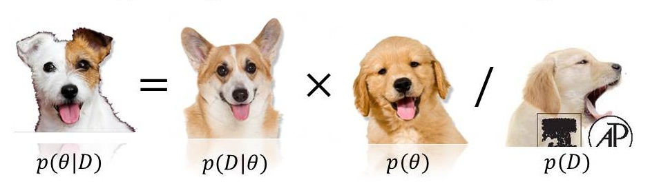
Bayes' puppies
posterior is a "compromise" between prior and likelihood
\[\underbrace{P(\theta \, | \, D)}_{posterior} \propto \underbrace{P(\theta)}_{prior} \ \underbrace{P(D \, | \, \theta)}_{likelihood}\]
influence of sample size on posterior

influence of sample size on posterior

highest density intervals
highest density interval
given distribution \(P(\cdot) \in \Delta(X)\), the 95% highest density interval is a subset \(Y \subseteq X\) such that:
- \(P(Y) = .95\), and
- no point outside of \(Y\) is more likely than any point within.
dummy
Intuition: range of values we are justified to belief in (categorically).
caveat: NOT the same as the 2.5%-97.5% quantile range!!
examples

example
observed: \(k = 7\) successes in \(n = 24\) flips;
prior: \(\theta \sim \text{Beta}(1,1)\)

the road ahead
BDA more generally
problems:
- conjugate priors are not always available:
- likelihood functions can come from unbending beasts:
- complex hierarchical models (e.g., regression)
- custom-made stuff (e.g., probabilistic grammars)
- likelihood functions can come from unbending beasts:
- even when available, they may not be what we want:
- prior beliefs could be different from what a conjugate prior can capture
dummy
solution:
- approximate posterior distribution by smart numerical simulations
fini
outlook
Tuesday
- introduction to MCMC methods
Friday
- introduction to JAGS
to prevent boredom
obligatory
prepare Kruschke chapter 7
finish first homework set: due Friday before class