- get in touch with R for
data wrangling & plotting
- think about data & its format
- manipulate data into appropriate format: data wrangling
- extract data summaries
- choose aspects to visualize data
- look at data set from case study on quantifier some

read more
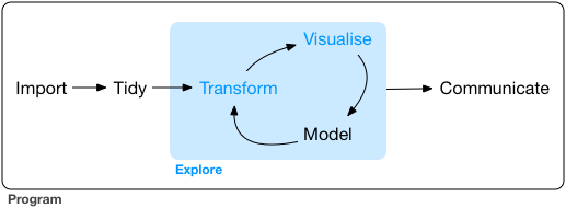
from R for Data Science
special purpose programming language data science
statistical computing
authority says to tell you: do not think of R as a programming language!
is a trusted old friend
a lot of innovation and development takes place in packages
install.packages('tidyverse')
library(tidyverse)
base R functionality is always available
rnorm(n = 5, mean = 10) # 5 samples from a normal with mean 10 & std. dev. 1 (default)
## [1] 10.611982 10.138658 10.025993 9.268167 9.181465
packages bring extra functions
library(mvtnorm)
mvtnorm::rmvnorm(n = 5, mean = rep(10,5)) # 5 samples from a multivariate normal
##           [,1]      [,2]      [,3]      [,4]      [,5]
## [1,]  8.848755  9.459086  9.212209 11.025298 10.782896
## [2,] 11.004074  8.563577  7.770695 11.474569  9.209217
## [3,] 11.629314 10.167166 10.143578  9.107262  9.785214
## [4,] 11.871819 10.113441 10.280624  8.931763 12.570017
## [5,]  9.172942  8.995465  8.879740 10.580737  9.776681
help('rmvnorm')
Mvnorm {mvtnorm}    R Documentation
Multivariate Normal Density and Random Deviates

Description

These functions provide the density function and a random number generator
for the multivariate normal distribution with mean equal to mean and
covariance matrix sigma.

Usage

dmvnorm(x, mean = rep(0, p), sigma = diag(p), log = FALSE)
rmvnorm(n, mean = rep(0, nrow(sigma)), sigma = diag(length(mean)),
    method=c("eigen", "svd", "chol"), pre0.9_9994 = FALSE)
integrated develop environment for R

this course will focus (entirely?) on rectangular data
not covered:
library(nycflights13)
nycflights13::flights
## # A tibble: 336,776 × 19
##     year month   day dep_time sched_dep_time dep_delay arr_time
##    <int> <int> <int>    <int>          <int>     <dbl>    <int>
## 1   2013     1     1      517            515         2      830
## 2   2013     1     1      533            529         4      850
## 3   2013     1     1      542            540         2      923
## 4   2013     1     1      544            545        -1     1004
## 5   2013     1     1      554            600        -6      812
## 6   2013     1     1      554            558        -4      740
## 7   2013     1     1      555            600        -5      913
## 8   2013     1     1      557            600        -3      709
## 9   2013     1     1      557            600        -3      838
## 10  2013     1     1      558            600        -2      753
## # ... with 336,766 more rows, and 12 more variables: sched_arr_time <int>,
## #   arr_delay <dbl>, carrier <chr>, flight <int>, tailnum <chr>,
## #   origin <chr>, dest <chr>, air_time <dbl>, distance <dbl>, hour <dbl>,
## #   minute <dbl>, time_hour <dttm>
study Chapters 5 and 12 from R for Data Science

"Some of the circles are black."


dummy

d = readr::read_csv('../data/00_typicality_some.csv') # from package 'readr'
## Parsed with column specification:
## cols(
##   id = col_integer(),
##   language = col_character(),
##   rt = col_integer(),
##   type = col_character(),
##   response = col_integer(),
##   nr_black = col_integer(),
##   variant = col_character(),
##   comments = col_character()
## )
d
## # A tibble: 5,112 × 8
##       id language    rt   type response nr_black variant comments
##    <int>    <chr> <int>  <chr>    <int>    <int>   <chr>    <chr>
## 1      1  English  3930 filler        1        5       C       No
## 2      1  English  3108   most        0        5       C       No
## 3      1  English  2599 filler        1        8       C       No
## 4      1  English  4405   many        1        7       C       No
## 5      1  English  2574   some        1        6       C       No
## 6      1  English  1917 filler        1        3       C       No
## 7      1  English  2471 filler        0        3       C       No
## 8      1  English  2495   many        0        6       C       No
## 9      1  English  2093   some        1        9       C       No
## 10     1  English  1767 filler        0        2       C       No
## # ... with 5,102 more rows
levels(factor(d$comments))[1:20]
##  [1] "bonuses always help with a toddler in the home ;)"
##  [2] "Cheers."
##  [3] "cool!"
##  [4] "Easy HIT thanks!"
##  [5] "Everything worked fine, thanks"
##  [6] "fun"
##  [7] "Fun and interactive. Thank you!"
##  [8] "fun fun fun"
##  [9] "Fun study"
## [10] "Fun study, thanks"
## [11] "fun survey"
## [12] "Fun, thanks!"
## [13] "good hit"
## [14] "Good luck with your research!"
## [15] "great hit"
## [16] "Great hit, good luck with your research."
## [17] "Great HIT!"
## [18] "Great survey. Thank you!"
## [19] "Hi"
## [20] "I accidentally clicked \"false\" on one of the \"some are black\" statements.  It was the one where around half were black"
table(d$language)
##
## American English          Egnlish          Enblish         Englashi
##                8               13                8                8
##          english          English          ENGLISH          englsih
##             2410             2457              103               26
##          englush         Enlglish           FRENCH         Japanese
##               13                8               13                8
##          Russian          Spanish            Tamil            white
##                8                8                8               13
d = dplyr::filter(d, ! language %in% c("FRENCH", "Japanese", "Russian", "Spanish", "Tamil", "white"))
table(d$language)
##
## American English          Egnlish          Enblish         Englashi
##                8               13                8                8
##          english          English          ENGLISH          englsih
##             2410             2457              103               26
##          englush         Enlglish
##               13                8
d = d %>% dplyr::filter(type == "some") %>%
          dplyr::select(-language, -comments, -type)
d
## # A tibble: 1,449 × 5
##       id    rt response nr_black variant
##    <int> <int>    <int>    <int>   <chr>
## 1      1  2574        1        6       C
## 2      1  2093        1        9       C
## 3      1  2543        1        3       C
## 4      2  1857        4        5       B
## 5      2 11454        4       10       B
## 6      2  2053        4        3       B
## 7      3  1479        1       10       D
## 8      3  1640        0        0       D
## 9      3  1199        1        7       D
## 10     4  4828        6        6       B
## # ... with 1,439 more rows
d = d %>% dplyr::rename(condition = nr_black)
d
## # A tibble: 1,449 × 5
##       id    rt response condition variant
##    <int> <int>    <int>     <int>   <chr>
## 1      1  2574        1         6       C
## 2      1  2093        1         9       C
## 3      1  2543        1         3       C
## 4      2  1857        4         5       B
## 5      2 11454        4        10       B
## 6      2  2053        4         3       B
## 7      3  1479        1        10       D
## 8      3  1640        0         0       D
## 9      3  1199        1         7       D
## 10     4  4828        6         6       B
## # ... with 1,439 more rows
d = d %>% dplyr::mutate(dependent.measure = ifelse(variant %in% c("A", "B"), "ordinal", "binary"),
                        alternatives = factor(ifelse(variant %in% c("A", "C"), "present", "absent"))) %>%
          dplyr::select(- variant)
d
## # A tibble: 1,449 × 6
##       id    rt response condition dependent.measure alternatives
##    <int> <int>    <int>     <int>             <chr>       <fctr>
## 1      1  2574        1         6            binary      present
## 2      1  2093        1         9            binary      present
## 3      1  2543        1         3            binary      present
## 4      2  1857        4         5           ordinal       absent
## 5      2 11454        4        10           ordinal       absent
## 6      2  2053        4         3           ordinal       absent
## 7      3  1479        1        10            binary       absent
## 8      3  1640        0         0            binary       absent
## 9      3  1199        1         7            binary       absent
## 10     4  4828        6         6           ordinal       absent
## # ... with 1,439 more rows
d = d %>% mutate(response = purrr::map2_dbl(dependent.measure, response,
                                            function(x,y) { ifelse(x == "ordinal", (y-1)/6, y) } ))
d
## # A tibble: 1,449 × 6
##       id    rt  response condition dependent.measure alternatives
##    <int> <int>     <dbl>     <int>             <chr>       <fctr>
## 1      1  2574 1.0000000         6            binary      present
## 2      1  2093 1.0000000         9            binary      present
## 3      1  2543 1.0000000         3            binary      present
## 4      2  1857 0.5000000         5           ordinal       absent
## 5      2 11454 0.5000000        10           ordinal       absent
## 6      2  2053 0.5000000         3           ordinal       absent
## 7      3  1479 1.0000000        10            binary       absent
## 8      3  1640 0.0000000         0            binary       absent
## 9      3  1199 1.0000000         7            binary       absent
## 10     4  4828 0.8333333         6           ordinal       absent
## # ... with 1,439 more rows
d %>% dplyr::group_by(dependent.measure) %>%
      dplyr::summarize(mean.response = mean(response))
## # A tibble: 2 × 2
##   dependent.measure mean.response
##               <chr>         <dbl>
## 1            binary     0.7854077
## 2           ordinal     0.6002222
resp.summary = d %>% dplyr::group_by(dependent.measure, alternatives, condition) %>%
                     dplyr::summarize(mean.response = mean(response))
resp.summary
## Source: local data frame [44 x 4]
## Groups: dependent.measure, alternatives [?]
##
##    dependent.measure alternatives condition mean.response
##                <chr>       <fctr>     <int>         <dbl>
## 1             binary       absent         0    0.09090909
## 2             binary       absent         1    0.47826087
## 3             binary       absent         2    0.77777778
## 4             binary       absent         3    0.95833333
## 5             binary       absent         4    0.96428571
## 6             binary       absent         5    1.00000000
## 7             binary       absent         6    0.93750000
## 8             binary       absent         7    0.98000000
## 9             binary       absent         8    0.92857143
## 10            binary       absent         9    0.96666667
## # ... with 34 more rows
ggplot()

ggplot(data = resp.summary, aes(x = condition, y = mean.response)) +
  geom_point()

ggplot(data = resp.summary, aes(x = condition, y = mean.response, color = alternatives)) +
  geom_point()

ggplot(data = resp.summary, aes(x = condition, y = mean.response, color = alternatives)) +
  geom_point() + geom_line() + facet_grid( . ~ dependent.measure)

ggplot(data = resp.summary, aes(x = condition, y = mean.response, color = alternatives)) +
  geom_point() + geom_line() + facet_grid( . ~ dependent.measure) +
  xlab("number of black balls") + ylab("mean response") +
  scale_x_continuous(breaks = 0:10) + scale_color_manual(values = c("darkgrey", "firebrick"))


obligatory
prepare Kruschke Chapter 4
fill in CSV file and send it to Christian Adam
optional