Comparing null-hypothesis tests for binominal data

I taught a tutorial on Bayesian data analysis at KogWis-2016 today, which had a running example of a simple binomial coin flip scenario, by means of which I tried to highlight the conceptual differences between three ways of doing (something that may be called) “null-hypothesis testing”:

1. $p$-values (our good-old pals),
2. Bayes factors for nested model comparison, and
3. Kruschke’s ROPE-based parameter estimation approach.

While preparing this material, it occurred to me that, if I would sit in that tutorial, what I’d really want to ask is: “Okay, these are conceptually different, fine. But how often do they make different predictions?” To address this question, at least partly, I wrote a simple R script. It’s result are illuminating. So, let me share this. The script can be downloaded here. Here’s what it does.

Suppose we flip a fair coin for a fixed number of times, say, $N \in \{ 10, 100, 1000, 10000, 100000 \}$. We know that the true bias is $\theta = 0.5$, so we know the probability of each possible number of successes $k$, for fixed $N$, is $Binomial(k,N,\theta)$. Let’s loop over all possible $k$, for each $N$, and check what the three different approaches will give us as their assessment about the true null hypothesis $\theta = 0.5$. Weigh this by the actual frequency of each outcome, and retrieve the de facto probability of falsely rejecting the true null. (The script is flexible enough to let you play with the actual, true value of $\theta$ independently of the null hypothesis to be tested.)

Before lunging into the results, we should examine how exactly the three approaches behave. Well, null-hypothesis tests with $p$-values are clear. For each $k$ and $N$ we would just use a binomial test. E.g., for $k = 7$ and $N=10$ we get a $p$-value of:

binom.test(7, n = 10, p = 0.5)$p.value

## [1] 0.34375

and, as usual, we reject the null hypothesis if the $p$-value is below the magic mark $0.05$. This means that we already know how often this approach will falsely reject the true null: as $N$ grows this will converge to 5%. (It is below 5% for small $N$ because we are dealing with a discrete distribution.)

As for Bayes factors for nested model comparison, the script uses the Savage-Dickey method and counts Bayes factors of at least 6 as substantial evidence in favor of a model. The script looks at the null model with $\theta = 0.5$ and an alternative model, which has $\theta \sim Beta(0.5, 0.5)$. For our current puproses, we could say that this approach “accepts” the null if the Bayes factor in favor of the null model is at least 6, that it “rejects” the null if the Bayes factor in favor of the alternative model is at least 6 and that it is inconclusive otherwise.

Finally, let us also consider the approach to null-hypothesis testing suggested by John Kruschke, e.g., in his delightful textbook. This approach looks at the posterior distribution over $\theta$, given the data, and ask whether a so-called region of practical equivalence (ROPE) around the null-value $\theta = 0.5$, say $[0.5 - \epsilon, 0.5+\epsilon]$ has overlap with or enitrely lies within or contains the 95% credible interval of the posterior. Here, I chose $\epsilon = 0.01$ and a prior $\theta \sim Beta(0.5,0.5)$ like in the alternative model for the Bayes factor approach. For the purposes of our present little adventure, let’s say that the ROPE approach rejects the null hypothesis if the interval $[0.5 - \epsilon, 0.5+\epsilon]$ has no overlap with the 95% credible interval of the posterior.

Let us then look at how frequently a false rejection of the true null hypothesis would occur under each of these approaches for different sample sizes $N$.

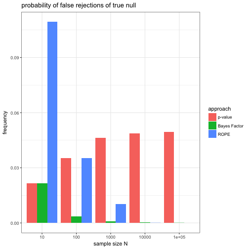
We see that, unsurprisingly, the $p$-value approach falsely rejects the null hypothesis at close to 5% of the time for larger and larger $N$. Interestingly, as $N$ grows, the Bayes factor approach seems to correctly not reject the true null almost always. Finally, the ROPE approach falsely rejects the true null remarkably often for small $N$. Based on the specifics of this set-up (e.g., $p$-value threshold 0.05, Bayes Factor threshold 6, ROPE’s $\epsilon=0.01$), we may conclude that the Bayes factor approach is most successful at avoiding falsely rejecting the true null. A more nuanced conclusion would be that both the $p$-value as well as the ROPE-based approach should ideally have thresholds ($p$-values and $\epsilon$) that are somehow sensitive to $N$. This echoes Lindley’s solution to the Jeffreys-Lindley paradox.

There’s much more room for exploration here, but for today, I’ll leave at that.